The 48 hr media cycle for the latest IPCC AR6 WG I) report is well past, but for anyone interested, here’s a short column with a few highlights in the Summary for Policymakers that caught my attention. The Summary plus full report are available here, https://www.ipcc.ch/report/ar6/wg1/
The Summary for Policymakers is 42 pages long and not that difficult to read for those with some science education.
The conclusions in the report are generally the same as in previous IPCC reports though with greater confidences for stated conclusions on climate change, and narrower projections of future temperature ranges. We’ll have more hot days, fewer cold ones, more intense rainfall events and higher evapotranspiration. Fewer tropical storms but more intense ones.
Global average temperature is now back up to the same peak reached about 6500 years ago. That agrees with what E.C. Pielou reported for Canada in her classic book, “After the Ice Age.” Of interest, Pielou also presented strong evidence that Western Canadian mountain glaciers largely melted at that time; what’s melting now with the current global warming are glaciers that mostly formed after peak temperatures 6500 years ago. (This is not to diminish the significance of present glacier loss to modern society.)
The new IPCC report places more emphasis than before, I think, on the cooling effect of aerosol compounds in the stratosphere (upper atmosphere). IPCC authors are quite confident that average temperature has increased about 1.1C since 1850-1900, but surprisingly uncertain on the extent to which this has been caused by GHG heating in the troposphere (lower atmosphere) and/or cooling by these upper atmosphere aerosols.
This part-sentence in Section A.1.3 is key, “It is likely that well-mixed GHGs contributed a warming of 1.0°C to 2.0°C, other human drivers (principally aerosols) contributed a cooling of 0.0°C to 0.8°C.” (“Likely” means 66% probability.)
This uncertainty also shows up in the IPCC WG I estimate of the warming caused by specified amounts of CO2 released into the atmosphere. In Section D.1.1, authors say, “Each 1000 GtCO2 of cumulative CO2 emissions is assessed to likely cause a 0.27°C to 0.63°C increase in global surface temperature with a best estimate of 0.45°C.” That’s a 2 1/2 times range in temperature response to given amount of CO2 emission, with a confidence level of just 66%.
IPCC projections on aerosol cooling also merit emphasis. If sulfur dioxide emissions decline with less coal burning and less air pollution, that could mean increased global warming because of less stratospheric cooling.
The net effect of the above, in my view, is some doubt about the precision of the IPCC’s projections of future temperature increases for given future amounts of GHG emissions. This is not to detract its overall message that human activities are causing global temperature changes and changing precipitation patterns compared to what would be expected solely from natural causes – and that a human priority should be to limit these changes to the extent possible while focusing also on adaptation.
I’ve one other comment: The IPCC report features five models of future climate changes to be expected with different levels of GHG emissions. But two of the five involve future rates of CO2 emissions far greater than what are being projected by most credible analysts – i.e., a 50% increase in rate of CO2 emissions by 2050 for one model and a near 100% increase by 2050 for the other. Discussions in the report of future climatic conditions with global warming are based too much, in my view, on these two unlikely models. Dr. Roger Pielke Jr. makes the same point though more eloquently and completely in a column here.
For those seeking more, here is one Twitter thread that I found very helpful: https://twitter.com/hausfath/status/1425504589097279494?s=20 . You should also consider following @Peters_Glen who posts meaningful analyses almost daily. The Breakthrough Institute (https://thebreakthrough.org/) also has published several good articles on climate change, of particular interest to agriculture.
As for what this means for global agriculture and food supply, I offer three conclusions:
Agriculture must devote more effort to technological changes, which reduce or even eliminate net GHG emissions, while still ensuring adequate supplies of nutritious food at reasonable costs for consumers.
Plant breeding and the use of advanced genetic technology, to produce new cultivars more resistant to heat and drought, will be even more important in years ahead.
Cultural techniques to store more water, including soil moisture reserves, from periods of intense rainfall for use during dry periods/seasons will become even more important than they already are.
This column was published originally in 2005 in the Ontario Farmer and is reproduced here with permission, for the interest and convenience of those interested in Ontario corn history.
Among the mostly forgotten chapters of Ontario corn history are many unsuccessful attempts to form an Ontario grain corn marketing board. The following description of these efforts is far from complete, but the best I could manage using various written records – often sketchy – and the living memories of individuals involved in the corn industry more than a half century ago.
The Ontario Corn Growers’ Association (OCGA) described in an earlier column was born in Essex County in 1908, in part because of a desire to promote the sale of seed of locally grown open-pollinated varieties, and died within a year or two after the formation of the Ontario Seed Corn Growers’ Marketing Board (OSCGMB) in 1940. The latter was created to represent growers of hybrid corn seed. Many of the farmers who were active in OCGA during the late 1930s became initial directors of the OSCGMB. The early history of the OSCGMB is described in Leonard Pegg’s “Pulling Tassels: A history of seed corn in Ontario,” published in 1988.
There was a parallel effort to create a marketing board for commercial grain corn. I know relatively little about the Essex-Kent Corn Producers’ Cooperative Association created in 1940 with Charles O’Brien of Roseland as president. However, a file in the Archives of Ontario describes how this organization promoted a proposed “Ontario Corn Growers’ Marketing Scheme.” The Essex-Kent cooperative group was created apparently to act as a central selling agency for marketing all commercial grain corn in southwestern Ontario. The group sought single-desk selling and compulsory government grading of all corn. There was major concern over low prices (40 cents/bushel), large harvest-time fluctuations in price, and a view that these were caused by inadequate competition. However, there is no record of a producer vote or widespread support.
Minutes of the Ontario Corn Committee (OCC, more detail here) show that representatives of the Essex-Kent cooperative group met with it in 1943 and 1947, mainly to discuss the importation of US seed corn and seed quality. Darrel Jubenville of Tilbury was a key spokesperson at these meetings.
The Ontario Archives also contain a proposal in 1946 by a group called the Commercial Corn Growers of Ontario to create “Corn Negotiating Committee” which would have the powers to negotiate minimum prices, grade standards, and associated shelling, elevation and handling fees with corn dealers and processors. The proposed membership of this Committee is similar to that of the earlier Essex-Kent cooperative association though the 1946 listing also includes representatives from Lambton, Middlesex, Norfolk, Elgin and Waterloo counties. The Archives contain copies of a ballot and draft letter to be sent to up to 7000 growers in April 1946. However, I can find no evidence that this mailing happened or that any vote occurred.
Darrel Jubenville and a few other farmers made group representations at various meetings of the OCC from 1948 through 1951. While they refer to the “association” which they represent, this association is not named in the OCC minutes.
More intriguing are Archive files from 1962 that include a March 6 letter from the secretary of the Ontario Farm Products Marketing Board to Deputy Minister Everett Biggs detailing procedures for a “recent Corn Vote.” The vote supposedly occurred between January 15 and 30 on the question: “Are you in favour of the proposed plan to be known as The Ontario Corn Producers’ Marketing Plan?” The Plan was to “1) provide a voice for growers, 2) develop markets and new uses for corn, and 3) promote corn for Ontario and Canada and ward off the inroads made by imports.” The vote was apparently championed by the Commercial Corn Growers Association led by Armould Mulcaster of Essex, with the support of the Ontario Federation of Agriculture, but was opposed by “The Five County Grain Corn Committee” led by Darrel Jubenville.
I can find no record of results of this vote or any indication other than the letter to Biggs that it even occurred. Certainly, no marketing board structure was created as a result.
In the late 1960s and early 1970s, agitation arose again among corn farmers for a marketing board to address low corn prices, then near $1/bushel. I recall meeting Jim McGuigan of Cedar Springs, then a director of the Kent and Ontario Federations of Agriculture and later the Member of Provincial Parliament for Kent-Essex. He told me of unsuccessful efforts by himself and many others to generate the support needed for a marketing board. “They’ll support marketing boards for nearly every other farm commodity,” said Jim in frustration, “but not for grain corn.”
However, because of producer discontent, Bill Stewart, the Ontario Minister of Agriculture and Food, called for a meeting of corn industry representatives to be held at the Ridgetown College of Agricultural Technology in September 1971. I was privileged to be present. (Darrel Jubenville and Mac Best from Fingal were also there representing the Canadian Commercial Corn Growers Association – the last written reference I’ve found to that organization.)
Delegates at the Ridgetown meeting recommended that an Ontario Corn Council be formed. The Ontario Grain Corn Council (OGCC) was officially created by Minister Stewart in December 1971 with Ken Patterson of Middlesex County serving as chairman, and eleven other appointed members. Ken served as chairman until 1986 and during this time the council effected a number of improvements including reduced rail shipping rates and tax incentives for new grain storage. The council actively promoted improved corn quality and the increased industrial processing of Ontario corn. It organized several export trade missions and helped create a Winnipeg Board of Trade futures market for grain corn with Montreal being the “delivery point.” (This market ended after about two years because of a lack of business.) Most importantly, the council portrayed corn as a major Canadian crop, and not just a regional grain grown mainly for on-farm feeding – the previous image. The council continued until about 1990 when the Ontario government ended its funding.
Creation of the OGCC did not end the pressure for a producer organization. Indeed, a group called the Corn Producers’ Investigating Committee from Kent County (chaired by Stuart Shaw but with Darrel Jubenville also present) met with the OGCC and representatives of the Ontario Ministry of Agriculture and Food (OMAF) in April 1972 seeking an “Ontario Corn Industry Act” and an associated board to provide much greater regulatory control over marketing and pricing. This proposal received no support from the council nor Minister Stewart. Dramatic increases in corn prices beginning in late 1972 were probably why pressure for a marketing board ended at that time.
Finally, in 1979, some corn growers began to work on plans for a new producer organization. The Ontario Corn Producers’ Association (OCPA) was founded in December 1982. Passage of the Ontario Grain Corn Marketing Act in 1984 gave OCPA checkoff collection powers, and it persisted until 2010 – then becoming part of the amalgamated group, the Grain Farmers of Ontario. OCPA was created without a producer vote, but with benefit of a refundable checkoff on producer grain corn sales to commercial buyers. It had no regulatory power over any aspect of marketing, only the power of lobbying and rational advice to governments. A more detailed column on the history of the Ontario Corn Producers’ Association will follow.
No-till soybeans planted in between rows of corn stalks
This overview is intended for those in Canadian agriculture interested in using proven, or partially proven, technologies to reduce net greenhouse gas (GHG) emissions through changes in farming practices.
If you don’t want to read further, my conclusions are: Opportunities look greatest for reductions in nitrous oxide (N2O) emissions. Further reductions in carbon dioxide (CO2) emissions through more usage of no tillage are possible, and the potential to sequester soil organic carbon through increased perennial forage production exists, but it’s questionable that these will lead to sizable futures decreases in national GHG emissions. Cover crops, with a few exceptions, probably represent limited opportunity for soil C sequestration in Canada with our long winter and short off-season growing intervals, but may prove more valuable for reducing spring-time N2O emissions. Future reductions in methane (CH4) emission are dependent on the extent to which promising research on rumen additives can be implemented in practice.
Carbon Dioxide
Let’s start with CO2 because, globally and nationally, it’s the most important of the three major GHG gases.
(The three gases are CO2, N2O and CH4. When GHG emissions are reported as CO2, that means only the one gas, but when reported as ‘CO2 equivalent,’ or CO2e, that means the collective warming potential of all three gases – plus a few more gases unrelated to agriculture that have smaller effects – all weighted for their relative potential to affect global warming. N2O has about 298 times the warming potential of CO2 on a per-kg basis; for methane it’s about 25, calculated as the average 100-year effect.)
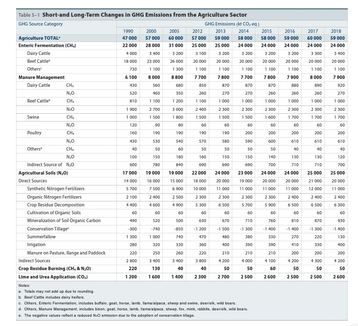
According to GHG accounting protocols specified by the International Panel on Climate Change (IPCC), agriculture represents 8.1 % of total Canadian emissions, but with CO2 only representing 4% of that. These stats are as reported by Environment and Climate Change Canada (ECCC) in its latest National Inventory Report (NIR) to the United Nations Framework Convention on Climate Change (UNFCCC). I’ve summarized Canadian data for 2018 here; the numbers for 2019 are virtually the same – ECCC 2019 summary here – entire report available here.
However, CO2 emissions associated with on-farm fossil fuel usage, biofuel manufacture/usage and net CO2 exchanges between farm soils and the atmosphere are not included in the NIR/UNFCCC calculations for agriculture. If these were in, the Canadian net agricultural emissions would represent 8.5% of the Canadian total (calculations here). Even with these additions and subtractions, CO2 still represents a very small percent of total net agricultural emissions.
If we go further and add GHG emissions associated with fertilizer manufacture (mainly N), the 8.5% grows to about 12%, with most of the increase being CO2, but with CO2 still being a relatively small portion of the Canadian agricultural total.
Finally, if the amount of carbon contained in products that leave Canadian farms and are exported were to be included, the total net GHG emission from Canadian agriculture would actually be negative – removal of CO2 from atmosphere exceeding all forms of ag GHG release. But that calculation remains far from IPCC calculation plans, at least as it appears now.
For the following discussion, I’ll focus only on two categories, net GHG exchanges for ‘Agriculture’ as reported by NIR/UNFCCC, and the agricultural soil portion of another category called, ‘Land Use, Land Use Change and Forestry,’ or LULUCF.
The Canadian NIR recognizes three sources/sinks for CO2 in its LULUCF calculations for agricultural soils. These are: land converted to continuous crop production from periodic summer-fallowing, land converted to reduced tillage and no tillage from more intensive tillage, and land converted into perennial forage production from annual crop production, as well as the reverses.
Emission factors for these land-use changes reported in the Canadian NIR are shown in Table 1 (taken from Table A3.5-8 in Part 2 of Canadian 2020 NIR).
Table 1. Effective linear coefficients of soil organic carbon for land management changes (LMC); for the opposite changes – eg., no tillage to intensive tillage – the linear coefficients are negative of the values shown in column 3.
Of the three factors, the largest effect by far comes from a conversion of annual crop to perennial cropping. Unfortunately, the trend in recent years has been more of the reverse – perennial to annual – a result of better prices for annual crops and declining beef production in some provinces.
An increase in perennial crop acres, ideally as part of crop rotations with annual crops, would be very beneficial for soil organic carbon sequestration, but it is difficult to see how this will happen – given increasing public interest in plant-based (that generally means annual-crop-based) alternatives to ruminant meat. A fledgling cash-crop industry is developing in Ontario and perhaps other provinces for the production and export of high-quality alfalfa hay, but the scale is still too tiny to permit conclusions on whether this will grow to represent a significant means for increasing SOC on a national scale.
The shift from intensive to no tillage provides the smallest per-ha annual change. Table 1 may over-estimate the no-till benefit in Atlantic Canada, Ontario and Quebec. Available research data are inconsistent as to whether there is a net positive no-till effect on soil organic carbon in this part of Canada. Research data show a more consistent increase in soil organic carbon with tillage elimination in the Prairie Provinces. But the biggest shift in Prairie crop acreage to no tillage may already have occurred.
A reduction in summer fallowing causes a larger per-ha annual effect than no tillage, but this is largely limited to the semi-arid Prairies where summer fallowing is still practiced to a significant extent – and this benefit declines as the portion of Prairie farm land available for summer-fallow elimination continues to shrink.
It must also be noted that the annual SOC sequestration provided by these changes in land management declines each year as shown below in Fig 1, extracted from the 2020 Canadian NIR. After 20-25 years, about 50% of the total GHG sequestration potential from a change in land management practice has been achieved.
Fig I. Changes in SOC sequestration with time after implementing changes in land management practices (from Fig A3.5-14 in Part 2 of Canadian2020 NIR). The dashed line denotes an annual sequestration of 25 kg/ha of SOC; once the estimated sequestration falls below this, the values are not included in Canadian LULUCF totals.
A popular means of sequestering soil organic carbon may be cover crops – at least as expressed at farm meetings and as featured in ag media of late. A number of global research publications also make this claim. However, in a recent review of the published evidence, I concluded that the likelihood for such is very limited in short-growing-season environments like Canada. There are exceptions – for example, red clover spring seeded into winter wheat, or for some horticultural crops where the off-season available for cover crop growth may be unusually long. Though I’d love to be proven wrong, I personally don’t see cover crops as a nationally significant option for CO2 sequestration. That may be the reason why cover crops are not included in the listing shown above in Table 1 taken directly from the Canadian NIR.
There is a strong alternative opinion to what I’ve expressed above. For one example, see this backgrounder written by the respected Dr. Brian McConkey (formerly with Agriculture and Agriculture Canada – AAFC – and now chief scientist with Viresco Solutions) for Farmers for Climate Solutions (available here, check Chapter 2). Dr. McConkey’s view is that a portion of any organic matter addition to the soil, no matter how small, contributes to SOC enhancement. That includes cover crops which may only produce a few hundred kg/ha of organic matter per season. His perspective may stem from this article written by Dr. Fan and a number of AAFC researchers including Dr. McConkey who conclude, based on computer models, that more organic matter addition to soil automatically means increased SOC content. However, the Fan article includes a series of graphs (Fig 5 in the paper, if you are looking) that predict, based on this perspective and these models, that the SOC percentage in farm soils of Southern Ontario should increase anytime the annual organic carbon addition exceeds about 3-4 tonne/ha.
But the annual organic matter addition to soil with a typical corn-soybean or corn-soybean-wheat rotation is about 12 t/ha – which equates to 5 t/ha (assuming organic matter is 42% C) and yet the SOC content of Ontario farm soils in principal cash crop areas of the province is in decline. See following graph courtesy of Christine Brown, Ontario Ministry of Agriculture, Food and Rural Affairs (OMAFRA), that is based on thousands of soil samples tested in Ontario labs.
There has to be more to SOC enhancement than just more added organic matter (not that the latter is not also important).
This paper containing results of a 10-year, multi-site study in Iowa provides an explanation. While the addition of organic matter including cover crops to soil will add additional organic matter, it can also increase the rate at which soil organic matter is respired – often resulting in no net gain in SOC.
McClelland et al 2020 in a meta-review found that SOC enhancement with cover crops was generally only significant when the annual cover crop dry matter accumulation was 7 t/ha or higher. Many cover crops in Canada produce only about a tenth of that.
In brief, while cover crops in certain situations may increase SOC, it is doubtful that collectively these represent an important opportunity to increase the carbon dioxide sequestration in Canadian farm soils. This is not to detract, at all, from other cover crop benefits, including important reductions in soil erosion.
Nitrous Oxide
The quantity of nitrous oxide (N2O) emitted each year, globally or nationally, is small compared to CO2, but the warming potential of a tonne of N2O gas is about 298 times greater. N2O represents about 5.2% of total Canadian GHG emissions measured as CO2 equivalents, but agriculture represents 76% of that according to the Canadian NIR.
Although some of the agricultural N2O comes from manure storage before field application, about 86% comes from the application of N fertilizers to farm soils, both synthetic N fertilizers and manure. There are some excellent reviews including this one done by a group of researchers at the University of Guelph as well as this, this, this and this.
The research results are extensive and quite consistent:
Increased N application rates mean more N2O loss. Indeed, the simplest IPCC calculation protocol for estimating national N2O soil losses expresses loss as a fixed percentage of N applied. Research suggests that N2O loss actually increases exponentially with N application rate, meaning the last 10 kg/ha of applied N causes the biggest N2O loss on a per-kg basis. There have been numerous agronomic/economic studies of the most economical rate – complicated by large annual variations in both actual N losses and crop yields caused by differences in amount and intensity of rainfall. Rapidly increasing yields over time for some crops – corn and canola are examples – also complicate these calculations. How to provide the additional N without increasing N2O losses?
Fertilizer additives that slow the transformation of urea and ammonium forms of N fertilizer will reduce N2O emissions. The literature suggests an average of about 30% reduction with the combined usage of a urease inhibitor (slows urea transformation into ammonium) and a nitrogenase inhibitor (slows ammonium transformation into nitrates) for treatment of urea or UAN (urea plus ammonium nitrate) fertilizers. The reduction is also sizable, though less, with the usage of polymer-coated fertilizers.
Partial side-dress application of fertilizer N, as compared to full application of N at or before planting, does not appear to reduce N2O losses consistently as a percent of N applied. But because side-dressing reduces the total N application need, this means a reduction in N2O loss. A lot depends on when intense rainfall events occur relative to time of application.
In a recent paper, Eagle and several co-authors from across the North American Corn Belt concluded that N2O losses are more closely related to the difference between N applied minus N removed in harvested crops, than to N application rate per se. This means that variable application rates based on within-field differences in measured late-spring soil nitrate levels or historic differences in within-field yield represent another good option for reducing N2O losses.
For a given rate of soil N addition, any practice that reduces soil nitrogen losses for other reasons, eg., reduced ammonia volatilization with fertilizer incorporation or reduced leaching loss of nitrate will often tend to increase N2O losses, so there are management tradeoffs.
N2O loss also tends to increase with Increases in soil organic matter content, so a tradeoff once again.
So what does all this mean? With the use of N fertilizer inhibitors, and adding combinations of partial side-dress N application and within-field variable N applications, it should be possible to reduce N2O losses by 30-50% or more with synthetic N fertilizer usage – with the cost for added technology being offset, at least in part, by lower average N fertilizer application rates.
Manure N seems more complicated. IPCC Tier 1 guidelines (the approach countries are to use in calculating GHG emissions when they lack the data or expertise to permit more sophisticated calculations) calculate a lower percent conversion of available N into N2O with manure compared to synthetic fertilizers. However, that is not well supported by North American research results that show that, on average, the two loss ratios are about equivalent. See references cited above.
To that, add the complication that manure is often applied to fields in the late summer or autumn – after wheat harvest, for example – to provide fertility for the crop to be planted the following spring. In provinces/states/countries – like Ontario – with substantial autumn and early spring rainfall, that can mean major N off-season losses via leaching, and N2O emissions.
Data summarized by OMAFRA indicate that 50 to 80% of the N content in late-summer/autumn–applied manure may be lost in off-season months. (The percentage varies across types of manure and whether incorporated or not.)
One solution is to apply manure in spring before or after crop planting but that can be logistically difficult in years with wet springs. Manure additives may reduce the problem though that’s a subject on which I have no knowledge.
Cover crops may sequester limited CO2 in Canada but could be very valuable for reducing early-spring N2O losses.
Cover crops are an opportunity to reduce emissions but this is a source of uncertainty. Research by Dr. Wagner-Riddle and colleagues at the University of Guelph (see publication here, and personal communication) has shown that early spring N2O emissions are significantly lower with a cover crop like winter rye. A substantial portion of the year’s total annual N2O emissions can occur during this short period; the cover crop effect seems to be one of reducing the depth of frost penetration, or maybe the number of early-spring freeze-thaw cycles.
However, other researchers at the University of Guelph hold a different opinion. “Conservation tillage, [and] cover cropping … increase N2O emissions,” state Ashiq et al (2021) as a highlighted conclusion in a recent review. My read of the literature indicates such an unqualified conclusion is probably inaccurate, though it likely reflects any effect of cover crops, if present during the main growing season, in preserving soil moisture and, hence, increasing the likelihood of anaerobic soil conditions for N2O formation.
Non-legume cover crops are well recognized for their value in reducing soil nitrate levels in autumn, and the expectation is that this will reduce the potential for autumn-winter-spring leaching losses. Cover crops may thus reduce the amount of nitrate available for N2O formation in early spring. But if the cover crop dies quickly following late-fall-early-winter frosts, thus releasing nitrates back into the soil profile in weeks to follow, this may mean more nitrate available for N2O formation in early spring – maybe even more than with no cover crop at all. Legume cover crops mean more soil nitrate availability and the potential for more N2O formation, especially at time of cover-crop death.
A very informative meta-review was published in 2014 by Basche et al. They found 29 relevant studies of paired comparisons – cover crop versus no cover crop. Of those, 40% found a decrease in N2O emissions with cover crop usage and 60% found an increase. In general, there was more likely to be an increase in N2O with cover crops when: the cover crop was an N-fixing legume versus grass/cereal or other species; the residues from killed cover crops were incorporated into the soil versus left on the surface; and when N2O emissions were measured during the initial time of cover-crop residue decomposition versus for longer periods of time. The reviewers also state that, to the extent that cover crops reduce nitrate losses from leaching, they will also reduce off-site N2O losses which can be substantial though not measured in any of the 26 studies.
A best option seems to be cover crops that remain fully viable over winter followed by no tillage so as to not incorporate residues. But getting them killed in time to not affect the growth and yield of the subsequent spring-planted crop can be a challenge – again especially in years with above-average spring rainfall. Dr. Eileen Kladivko of Purdue University provides a good discussion on these options here.
Cover crops may ultimately prove to be of much more value in reducing GHG emissions by suppressing N2O formation, than by sequestering soil carbon, but it is difficult to be certain at this time.
Methane
The greenhouse gas, methane (CH4), represents a much smaller quantity of global emissions than CO2, but provides a substantially higher ‘warming potential’ per tonne. Unlike N2O and CO2, CH4 has a relatively short half-life in the atmosphere (about 10 years) before being broken down into water and CO2 molecules. Methane represents about 13% of total CO2e emissions for Canada, according to IPCC-based calculations, of which about 31% comes from agriculture – and 86% of the 31% comes from ruminant digestion. There are a couple of key issues though I’ll spend limited time on them here as they are addressed well elsewhere, including here and here.
Beef cattle grazing. Photo courtesy Dr. Vernon Baron, Agriculture and Agri-Food Canada, Lacombe, Alberta
One involves the fact that IPCC calculations, based on average warming effects of GHG gases over 100 years do not work well for short-lived gases like methane, with its half-life of about 10 years. And based on an improved calculation procedure developed at Oxford University, the true long-term GHG effect of methane should be much smaller than in the numbers submitted by Canada and others in their annual NIR. This is especially true for Canada where methane emissions from ruminant livestock have been in decline for about the last 15 years. However, a related blog with analysis that I posted in September 2020 has generated about zero interest, and I’m not seeing much greater interest in related articles written by those with much stronger credentials and connections. I’m not optimistic that the work from Oxford U will result in any change in calculation protocol specified by IPCC for annual NIR submissions.
One problem is that the improved calculation methodology also applies to methane emissions associated with fossil hydrocarbons. That’s most of the 69% in Canada not represented by agriculture. This includes natural gas pipeline leaks. Politically, few in the environmental/climate-change lobby want to make changes that would be seen to benefit ‘Big Oil and Gas.’
The other issue involves the potential use of seaweed extracts and other rumen additives to reduce methane production. These technologies look very promising though are largely still at the ‘proof of concept’ stage of development. More R and D work will be required before they can be truly classed as a principal solution for reducing GHG/CH4 emissions associated with ruminant agriculture.
From a broader agricultural perspective, any technology that encourages beef/sheep production will also encourage greater use of perennial forage crops in Canadian farm crop rotations – with major benefits to soil quality and C sequestration opportunities.
Scope for Zero Emissions?
The focus of international discussion, at least in high-profile circles of late, is not so much strategies for partial reductions, but rather, for zero net emissions. Nations and corporation are both competing for media attention in announcing their new strategies for achieving zero emissions by 2050 or even sooner. The cynic in me doubts that most of these mean much as they depend on major future use of technologies that are far from proven, and/or calculations based on avoiding future GHG-producing practices (e.g., credits for not cutting down trees or draining swamps). They also depend on a level of political and public support which is not yet apparent.
So what’s the prospect for zero emissions in agriculture? I’m not aware of many attempts by main-stream agriculture to tackle this question but there are a few. I give credit below to two farm/agricultural groups that have attempted to develop/define strategies, even though I think that both have major flaws.
One is the National Farmers Union for England and Wales which, in this document, describes a strategy for achieving zero emissions from agriculture by 2040. The strategy is based in part on a national strategy developed by the Royal Society. In the NFU’s plan to eliminate the current emission total of about 45 Mt CO2e, it proposes to achieve about 25% of that by reductions in direct emissions of CO2, N2O and CH4 from farming; 20% by additional C sequestration in farm soils, fence rows, farm woodlots and wetlands; and about 55% by the combination of biofuel production/consumption coupled with the storage of CO2 released in ethanol manufacture using ‘carbon capture and storage’ (CCS) technologies (essentially underground storage of CO2, though the NFU leaves the door open to other CCS options).
It’s a big stretch to assume that either the sequestration or biofuel-CCS goals are achievable, but full marks to the NFU for offering something.
Another report is one done by the Aspen Institute in Colorado for the US Farmers and Ranchers Alliance (USFRA). The report, based in part on an analysis of negative emission and sequestration technologies by the National Academies of Sciences, Medicine and Engineering (it, in turn, based on an earlier report by Eagle et al), projects that US agriculture could reduce net GHG emissions by 147% by expanded use of technologies such as no tillage, cover crops, better grazing methods and use “frontier” technologies now in early stages of development. (USFRA, in a more recent report with the Foundation for Food & Agriculture Research and based on an analysis done by a team led by the Nature Conservancy, states that the potential offset is actually more than 200%, though with much of this coming from the management of new and existing forests on farmer-owned land.)
One problem with both the NFU and the USFRA proposals is that, even if the projected reductions were to be attained, most of them would not be credited to ‘Agriculture.’ Rather, the credits would go to other sectors such as ‘Energy’ (for biofuels) and Land Use and Land Use Changes (for C sequestration).
Using the present IPCC calculation methodology, one could offset 100% or more of agricultural emissions with soil carbon storage – as in the Aspen-USFRA calculations – and still have agriculture identified as the source of about 8-10% of national GHG emissions as at present. With the NFU strategy, 75% of the projected GHG reductions/offsets would not be credited to Agriculture.
In brief, while it may be important politically for agriculture to portray that it has plans to achieve zero emissions by mid-century (as the NFU has done), my conclusion is that this is not achievable using even semi-proven technology known today, and especially with current accounting procedures.
Bottom line:
Sizable opportunities exist now to reduce nitrous oxide emissions in agriculture using proven technologies, and with others looking promising – eg., selective use of cover crops to reduce N2O spring-time emissions. The potential for methane emission reduction is promising if new rumen-additive technologies prove feasible. The opportunities for C sequestration appear more limited unless means can be found for more greatly expanded use of perennial forages in farm crop rotations.
(This article is targeted mainly to Canadian farmers interested in climate change and greenhouse gas (GHG) emissions linked to agriculture.)
A coalition called Farmers for Climate Solutions (FCS) released its request on February 24 2021 for $300 million in Government of Canada money for a collection of programs to reduce GHG emissions in Canadian agriculture. I’ve reviewed their request and various background documents released at the same time. My comments follow.
First some background. FCS was launched in February 2020. It’s a coalition of some organic groups, the National Farmers Union of Canada (NFU) and some environmental NGOs. It says that it’s farmer-led but the primary leadership seems to come from Equiterre, a Montreal-based NGO.
FCS says it represents 20,000 farmers. What that likely means is that its component members have 20,000 members. It’s appears that the interaction between FCS and other major Canadian farm organizations, to date, has been minimal.
FCS seems to be well funded, backed by some major left-leaning foundations. Its web site and related materials are highly sophisticated and professionally done. Its release on February 24 was matched by a supportive opinion piece the same day in the Globe and Mail. FCS is clearly well connected; not many groups could arrange for that. I believe this is well beyond the expertise of the NFU or any of the organic organizational members.
That said, FCS leaders get good marks for an initiative that is badly needed – how to reduce GHG emissions associated with Canadian agriculture. They have stepped into a space largely left empty, until now, by main-stream Canadian farm groups. (I do note the formation of the Agriculture Carbon Alliance, a coalition of mainstream groups on March 1, 2021; this is a welcome initiative, though starting a full year after FCS.)
FCS created a task force which contains several Canadian scientists for whom I have high respect. And it does appear that the task force played a major role in developing FCS policy. I personally agree with a good portion of what they have stated and proposed. But I also have some major questions about the rationale, implementation processes and omissions.
FCS leaders and task force members identified six areas where they feel government money could be best spent to reduce agriculturally related greenhouse gas emissions in Canada. These are as follows:
Doing more with less nitrogen
Increasing adoption of cover cropping
Normalizing rotational grazing
Protecting wetlands and trees on farms
Powering farms with clean energy
Celebrating climate champions
The total ask is $300 million from Ottawa, plus another $115 million from Canadian farmers, for a total cost of $415 million.
Here are more specifics:
Doing more with less nitrogen
FCS has provided a well-written, well-researched background report on factors affecting nitrous oxide (N2O) emissions from soils and the application of synthetic fertilizers (though not manure). The information is very similar to that provided in this report by Dr. Claudia Wager-Riddle, Dr. Alfons Weersink and colleagues at the University of Guelph. The FCS report divides Canadian farmers into just three groups based on assumed adoption of the “4R” strategy for responsible nitrogen management. I found this to be rather simplistic, given the wide diversity of Canadian agriculture and growing conditions.
Based on this report FCS recommends that Canada spend $115 million matched by a similar expenditure by farmers over two years. FCS documentation states that this money will be mainly used to hire a large number of agronomists to educate farmers on better N application procedures, to take a soil sample per farm to test for nitrates at the season end, and to take leaf tissue samples. My understanding is that this is to happen in 2022 and 2023.
However, my personal discussion with FCS indicates that their intent is actually broader with money being used to implement N2O reduction measures as well as just monitoring. That makes more sense to me as I cannot see how end-of-season nitrate testing, per se, will tell much until it has been done for several years and at several locations per farm, given the large variation in measurements expected because of locational and seasonal differences. Soil nitrate levels at season end depend strongly on annual differences in soil organic matter mineralization (conversion to inorganic N), weather and crop yields as well as fertilizer applications. Similar complications apply to leaf measurements of nitrogen content, with the genetic influence being very important.
Interestingly, the FCS analysis and plan resembles in several ways a strategy for N2O reduction that was developed by the Canadian Fertilizer Institute (CFI) 10 years ago. (Link is here.) I understand that this initiative did not proceed because of a lack of financial support by all Canadian governments except Alberta.
Perhaps there is opportunity to connect what FCS is proposing, including its major request for public funding, with what CFI has proposed. To add to that, I cannot see how the FCS strategy can be implemented in such short time frame without close integration with the sophisticated and extended network already existent with regional agronomists – most of them private and most being Certified Crop Advisors (see here and here).
The CFI plan as well as the scientific analysis in the FCS backgrounder both emphasize the value of slow-release forms of N fertilizer including urease and nitrification inhibitors and variable-rate-within-field N applications. That would be an excellent place to target government incentive money in my view. There may also be opportunities to reduce overall N application rates though one needs to be careful of analyses based on older crop data – given how crop yields, especially for corn and canola have risen so rapidly in recent years – and where calculations of optimum rates are based after the fact using knowledge of the weather that occurred during the crop growth season.
Increasing adoption of cover cropping
A background science-based analysis is provided to justify the expenditure of $115 million over two years to provide incentives for cover crop establishment. I am quite happy to see the government spend money encouraging cover crop usage as cover crops provide many benefits. However, I don’t believe that one of those benefits is nationally significant increases in soil organic carbon content (SOC), given Canada’s mostly cool/cold seasonal conditions – especially with the field crops which currently occupy most arable land acreage. My rationale, based on a review of many scientific reports and meta-reviews, is posted here.
With all due respect to the FCS task force members, I don’t think their scientific backgrounder on cover crops is very convincing. It’s in distinct contrast to the discussion on N2O. The FCS backgrounder cites three studies to support its claim that cover crops enhance SOC. I’m familiar with all three. Of them, one shows no statistical difference in SOC between soils with or without various types of cover crops, one states its data cannot be used for conclusions about soil C sequestration because of the lack of soil bulk density data, and the third made up for the lack of bulk density data by using data from other studies, sometimes even on other continents, while also including studies where the ‘cover crop’ was the only crop grown all season. The task force report does note that its estimates are often based on “limited evidence” and “expert opinion.” Core calculations for Canada are based essentially on very simplistic and speculative calculations. But then the report provides a series of quite detailed tables listing sequestration potential for various agricultural zones and crop species, including offsetting N2O emissions – giving the appearance of precision where such is not justified, at least in my humble opinion.
However, to repeat: I’d be happy to see a program providing inducements for cover crop planting. But the proposed cost is rather high – $115 million over two years – and its promise of GHG emission reductions of 2.2 Mt of CO2 equivalent seems highly speculative and unlikely.
I am suspicious that FCS leaders view this as a program to promote cover crops per se. There is an emphasis in the project description to the differential channeling of money on a per-acre basis to small farmers while making sure that the big guys don’t get too much. If your purpose is to reduce GHG emissions then an acre is an acre, and individual farms with large acreages would seem a priority target. But if your goal is some money to every farmer to plant some cover crops, then money per farmer rather than per acre is more attractive.
Normalizing rotational grazing
The request here is smaller – $25 million (but still large – perhaps exceeding the entire research budget of Agriculture and Agri-Food Canada devoted to GHG reduction). The rationale is a mixture of better management of rangelands in Western Canada and introduction of other crop species into managed pastures. I don’t have enough background to judge the potential effectiveness of what they propose. However, I wish their analysis and purview had stretched further, to include the expanded use perennial forages in Canadian cropping programs. The Government of Canada National Inventory Report submission to the United Nations identifies more perennial forages as about the best way to increase SOC content on Canadian crop land. (For details see the 2020 Canada National Inventory Report, Part 2, Table A3.5-8; link is here.)
The FCS report completes ignores broader aspects of ruminant grazing/agriculture on GHG emissions such as methane emissions associated with forage digestion, and methane and N2O from manure. Indeed, the FCS report seems to ignore animal agriculture completely even though it represents about half of total Canadian GHG emissions, at least as calculating using protocols of the IPCC (International Panel on Climate Change, United Nations).
Personally, if I had $25 million to invest in this general area, I would devote it to more perennial forage production and the developing (and exciting) new usage of new feed additives to reduce methane emissions from ruminants.
Protecting wetlands and trees on farms
This item promises a mitigation of 4.1 Mt of CO2 equivalent for an expenditure of $30 million. As I understand it, this is to pay farmers not to cut down woodlots and drain wetlands. The 4.1 Mt is not new sequestration but rather loss which might occur with tree removal and wetland draining.
The rationale is a bit hard to understand from an Ontario perspective in that we already have extensive laws to prevent forest removal and wetland draining (i.e., wet land being land that is water logged for a substantial portion of the year and not just for an extra week or two at time of spring planting). It’s true that these vary significantly across municipalities. However, I would argue that an expanded regulatory approach makes more sense nationally, rather than what would need to be continual payments to farmers to prevent destruction. $30 million would not go far in protecting all existing woodlots and wetlands – ideally grasslands too – on Canadian farms and ranches
Note this recommendation from FCS is in addition to the $3 billion that the Government of Canada committed to tree planting in its GHG policy announcements in December 2020.
Powering farms with clean energy
An expenditure of $10 million over two years for an unstated GHG benefit.
The money would be spent for retrofitting 100 diesel tractors per year and use of electric-powered tractors on small farms.
All modern diesel farm tractors have highly efficient emission control systems which outsiders (including farmer owners) are prohibited from doing much more than changing the oil. More usage of electric tractors will come but it’s not clear how this $10 million investment in Canada will make any difference.
One of the biggest opportunities for reducing farm tractor fuel consumption is via reduced or no tillage. That is not mentioned here. I understand why this might be a sensitive subject for FCS with its organic farm membership, and for whom frequent tillage is the norm. But better to focus on how to get organic farmers to till less – or not at all – and even feature technologies which discourage tillage usage like the use of glyphosate for vegetation control – rather than avoid the subject in the FCS report. To be fair, I note that options for reducing tillage are one of the current priority goals for several Canadian organic organizations.
Most critically, this section of the FCS report completes ignores biofuels and the Clean Fuel Standard (CFS) announced by the Government of Canada in December. A calculation that I did using data published in the Government of Canada National Inventory Report of April 2020 indicated that the use of biofuels now means a reduction of 6 Mt CO2 equivalent per year for Canada, with more expected with CFS implementation (analysis here). That’s more than any of the six strategies proposed in the FCS document.
Celebrating climate champions
The FCS are requesting $5 million to provide awards to “showcase and amplify the voices of farmers who are charting the path for sector-wide change.” I am a bit nervous about this as I could see it being very political. There is a strong bent towards organic farmers in photos and mini-bios in the February 24 documents. Of course, that’s not surprising since this is an organic/NFU/Equiterre led initiative. But who chooses the farmers, and what might be the criteria – low emissions per acre where organic shines according to some published analyses – or low emissions per unit of food produce where organic is generally inferior?
I think the government could probably find better ways to use $5 million to reduce GHG emissions in agriculture. My vote would go for credible scientific research.
What did they miss?
To add to – and emphasis in some cases – what I’ve stated above, I believe the report has some notable voids. These include:
Reduced tillage/no tillage. The Government of Canada National Inventory Report on national GHG emissions highlights the value of no tillage agriculture for enhancing SOC. The benefit is much clearer and better documented for the Canadian Prairies than for BC and provinces east of Manitoba, but research data from the University of Guelph demonstrate that this benefit can be substantial for certain soil-crop combinations in Ontario too. I expect the same applies in Quebec and Atlantic Canada. Granted the annual benefit decreases with time as SOC increases, but the same applies for any other method of soil C sequestration (including cover crops to the extent that they provide this service). Current Canadian National Inventory Report statistics say that reduced tillage now means about a 4 Mt CO2 equivalent reduction in Canadian GHG emissions per year. (For more detail, see Table 6-9 here.) That’s larger than any item in the FCS list.
Livestock-related emissions. Reductions in GHG emissions through feed additives and manure management. About 30 Mt of CO2 equivalent emissions now occur because of ruminant metabolism and manure gases according to the National Inventory Report. There are good opportunities for reductions.
Great use of perennial forages in Canadian cropping, including opportunities for cash-crop production and marketing of crops like alfalfa. Several Ontario farmers including a farmer cooperative are already marketing high-quality forage produce in Asia.
Biofuels, building on the base outlined in the new Clean Fuel Standards of the Government of Canada. Biofuels mean about an annual 6 Mt reduction in CO2 equivalent net emissions currently. The potential is larger.
Next steps
The Farmers for Climate Solutions and its task force members are to be congratulated for their initiative in emphasizing the importance of strategies to reduce GHG emissions with Canadian agriculture and for drafting a proposal for steps forward. A logical next step would be for either FCS to engage with the 90%+ of Canadian farmers and farm sectors who are not part of the coalition to identify practical means for moving forward including opportunities not identified in the February 24 documents. Or an alternative is for main-stream agricultural groups to use what FCS has proposed as a base for developing their own proactive programs for reducing net GHG emissions.
I’ll start with a definition: I think most agriculturalists take ‘cover crop’ to mean a crop grown in the same year as a primary crop such as a harvestable grain or horticultural crop, and that’s what’s assumed in this article. As noted below, some authors also include crops grown alone for the full season, solely for soil quality enhancement.
Current enthusiasm within agriculture in cover-crop usage is well placed. These crops provide clear benefits in protecting soil from water and wind erosion, providing end-of-season livestock feed, enhancing biodiversity, supplying significant quantities of legume N fertility for use by subsequent crops, and removing nitrates from soil at the end of the growing season (though the fate of nitrates thereafter often remains uncertain).
In addition, major attention is being placed on the potential for cover crops to sequester photosynthetically fixed carbon dioxide (CO2) as soil organic carbon (SOC). This includes discussion on possibilities of paying farmers for doing this.
There have been many research trials completed and several meta-reviews published. This column contains a review of what the meta-reviews say individually and collectively – and what it means for agriculture and net greenhouse gas emissions, especially in a northern climate like Canada.
This article is written primarily for an agricultural audience interested in more depth than generally found in media and agricultural ‘extension’ reports, but less than in found in scientific papers. My column has not been peer reviewed although I have checked analytical details with several of the authors cited below.
I’ll start with my conclusions: The evidence is convincing that cover crops often mean more SOC. This benefit is largely proportionate to how long the cover crop grows, how much cover-crop organic matter is produced, and the average annual temperature of the location. A measurable effect is much less likely when the season of growth is short, e.g., when cover crops are seeded after longer-season harvestable crops and/or when the off-season consists of many months of frozen winter. Most authors assume that more SOC with cover crops means increased carbon sequestration, which is probably true in many cases. But the other possibility is reduced or no loss of soil organic matter when cover crops are present, as compared to soil with no cover crop.
That said, notable weaknesses are common in many of the research summaries, including:
Reports based very few years of cover cropping (sometimes only one).
The inclusion of data from experiments where the ‘cover crop’ was the only crop grown for an entire season – and, hence, not really a cover crop by the definition stated above.
The inclusion of experiments measuring percent SOC or soil organic matter only, with no data provided on soil bulk densities especially for cover-crop treatments in the studies. Procedures have been developed for estimating the missing bulk-density values, but these generally introduce sizable errors.
Different sampling depths within or among experiments – range from 2.5 cm to more than 100 cm (though few below 30 cm) – often with simple calculations used to ‘standardize’ to a common depth.
In addition, with one exception which included Chinese literature, none of the reviews included research reports written in languages other than English.
I’ll refer to these in turn as we look at the results of the various meta-reviews. I should emphasize in advance, that all of the reviews represent a huge amount of work, with authors making major efforts to adjust for weaknesses and inconsistencies in the data sources used. I am most appreciative of that. But at the same time, it’s fair to examine their conclusions in light of how the limitations are addressed.
Now to the specifics.
Eagle et al (2012) of the Nicholas Institute for Environmental Policy Solutions, Duke University, published Greenhouse gas mitigation potential of agricultural land management in the United States: A synthesis of the literature, which includes a chapter called Use winter cover crops. Thirty one field studies were examined with a calculated average annual soil organic carbon gain equivalent to 1.3t/ha/year of CO2 (range -0.2 to 3.2) or 0.35 t C/ha/year. However most of the data referenced in this review came from California and southeastern states. There were six comparisons from states further north, three from Iowa where the cover crop treatments actually caused a slight reduction in rate of soil organic C accumulation and three from Michigan with gains ranging up to 1.83 t/ha/year of CO2. The Michigan studies were comparisons of an organic rotation of corn-soybeans-wheat plus cover crops with conventional corn-soybeans-wheat grown without cover crops. When I checked publications/web-sites, cited in these publications as providing more details on methodology, I was unable to find some key details on organic practices used, specifically the source of N fertility. Was the fertility provided by manure or other organic amendments? I don’t know. Hence, I suggest viewing the Michigan results with caution.
Eagle et al also refer to a study from Maryland in which the percent organic matter was higher in a cover crop treatment; they did not include this study in their calculation of mean effects because there weren’t data on bulk density and quantities of soil organic C per unit soil surface area. A summary table published by Eagle et al includes three model calculations and one “expert opinion,” all projecting more SOC with cover crops.
In essence, the Eagle et al review shows consistently more soil organic C with cover-crop usage in southern states, but an uncertain-to-zero benefit in the US Midwest.
Poeplau and Don (2015) published Carbon sequestration in agricultural soils via cultivation of cover crops – a meta-analysis, with the analysis involving 30 studies, 37 sites and 139 plots. The studies were in 11 countries, including Canada and the United States, and across four continents. Number of treatment years ranged from one to 38 and sample depth from 2.5 cm to 120 cm though with only three studies having samples “below the plough layer.” They calculated an average rate of soil C accumulation in cover-crop treatments, compared to plots without cover crops, of 0.32 + 0.08 t/ha/year of organic C. This paper and this quantity have been cited many times in other publications in support of statements that cover crops increase soil organic carbon.
For no other apparent reason other than I’m Canadian, I chose to check details of the four cited studies which were from Canada. They are:
Campbell et al, 1991, Effect of crop rotations and cultural practices on soil organic-matter: microbial biomass and respiration in a thin black chernozem. Can. J. Soil Sci. 71, 363–376. A 30-year study in Saskatchewan
Curtin et al, 2000.Legume green manure as partial fallow replacement in semiarid Saskatchewan: effect on carbon fluxes. Can. J. Soil Sci. 80, 499–505. A nine-year study in Saskatchewan.
Hermawan and Bomke, 1997. Effects of winter cover crops and successive spring tillage on soil aggregation. Soil Tillage Res. 44, 109–120. A one-year study in British Columbia.
N’Dayegamiye and Tran. 2001. Effects of green manures on soil organic matter and wheat yields and N nutrition. Can. J. Soil Sci. 81, 371–382. A five-year study in Quebec.
Of the four studies, three (Campbell et al, Curtin et al and N’Dayegamiye and Tran) all involve ‘green-manure crops’ grown without any other crop for the growing season and not the definition of ‘cover crop’ given at the beginning of this column. I did not check the other 26 cited studies in this review, but it is quite possible that there are additional ‘green-manure’ studies of the same nature included in the analysis by Poeplau and Don.
A second concern for me with this review is that only 30% of the cited studies contained data on soil bulk density. The authors estimated bulk density values for the other 70% using the graph below copied from their paper. It is based on collective data from the 30% of experiments with bulk density data across all countries.
Ignoring the one outlier value (which seriously distorts the R2 and p calculations), the line looks like a reasonable fit for the other data. That notwithstanding, the values for bulk density predicted by the graph still appear to have a range of at least +0.05 g/cm3 for a given percent C content. For a soil horizon that is 22 cm deep and about 1.5% SOC, this range in bulk density equates to 3.3 t/ha of organic C, or about 10 times the predicted average accumulation rate of 0.32 t/ha/year advantage for cover-cropped plots.
A third unease for me involves the process used to standardize all organic C measurements to a depth of 22 cm using average measured or predicted bulk density for the assayed horizon – thus mathematically ignoring the normal tendency for SOC concentration to decrease with depth. One might argue a more sophisticated transformation process is not warranted given uncertainties introduced by the bulk density estimates. But it is still another source of imprecision.
In summary, in my view, results of the analysis by Poeplau and Don are sufficient to indicate that cover crops often mean a higher soil C content, but not nearly enough to merit a conclusion of a rate of gain of 0.32 + 0.08 t/ha/year.
As part of an extensive 2019 report called Negative emissions technologies and reliable sequestration, the National Academies of Science, Engineering and Medicine in the United States included a short section recommending cover crops as a means of sequestering soil carbon. However, it only cited two references, Eagle et al (2012) and Poeplau and Don (2015), the two reviews discussed above.
Mcdaniel et al (2014) published a meta-analysis entitled, Does agricultural crop diversity enhance soil microbial biomass and organic matter dynamics? It involved 122 publications with 454 observations. The review featured additional crops inserted into monocrop cultures or simple rotations, and a substantial number of the studies (I don’t think the authors don’t say exactly how many) involved cover crops. About two-thirds of the studies were from North America and the rest distributed globally. Because only 19% of the studies included measurements of soil bulk density to permit the calculation of soil organic carbon content per unit land area, Mcdaniel et al reported only the soil organic carbon concentrations. Because soil samples within individual studies sometimes came from different depths, Mcdaniel et al converted these to an average depth per experiment with no weighting for changes in bulk density with depth. (For their rationale, see Johnson and Curtis, 2001.) There was no adjustment to a common depth across studies.
Mcdaniel et al concluded the inclusion of cover crops increased the soil organic carbon concentration by 8.5% relative to plots with no cover crop. This was a much greater effect than for all other crop rotational comparisons combined in their analysis. The relative SOC boost with cover crops increased with increases in average annual temperature across the various research locations.
The authors defend their use of percent soil organic carbon (i.e., as g/g x 100%) instead of the use of soil organic carbon stocks (t/ha) by the presentation of an appendix graph showing no significant relationship between “% change from monoculture” and soil bulk density. It’s based, I believe, on observations from the 19% of surveyed studies that had bulk density data. Their assumption is in disagreement with the graph presented above from Poeplau and Don showing a trend for bulk density to decline as percent SOC increases.
If bulk density declines as percent SOC increases, this means changes in t/ha of SOM with cover crop addition would be expected to be less than the measured changes in percent SOC.
Kaye and Quemada (2017) in a paper entitled, Using cover crops to mitigate and adapt to climate change. A review, concluded that “Cover crop effects on greenhouse gas fluxes typically mitigate warming by ~100 to 150 g CO2e/m2/year” with “the most important terms in the budget [being] soil carbon sequestration and reduced fertilizer use after legume cover crops.” Their conclusion on carbon sequestration is based largely on the analyses done by Eagle et al (2012) and Poeplau and Don (2015), which are discussed above.
Norris and Congreves (2018) in a review entitled, Alternative management practices Improve soil health indices in intensive vegetable cropping systems: A review, identified 60 studies where various practices had been used in attempts to improve soil health. They selected 22 of these studies, 11 involving cover crops, for a meta-analysis. The meta-analysis revealed no significant relationship between the presence or absence of cover crops and SOC. (It is assumed that SOC is expressed as a concentration rather than t/ha or equivalent in this review, though I don’t believe the authors actually say so.)
Abdalla et al (2019) published a review entitled, A critical review of the impacts of cover crops on nitrogen leaching, net greenhouse gas balance and crop productivity. Using the Web of Science data base they chose 106 studies involving several key words including, ‘cover crop,’ ‘soil organic carbon’ and ‘SOC.’ The range was global but most studies were from the United States/Canada, Europe and China. The objectives of this meta-analysis included the dynamics of soil nitrogen as well as carbon. For questions about SOC, the authors selected the 47 studies containing data on SOC in t/ha (or equivalent) or the combination of percent SOC and bulk density so that SOC in t/ha could be calculated. The authors adjusted SOC data to a standard depth of 30 cm based on an assumption that SOC decreases with depth at a rate of 2.14% per cm of depth. The rationale for that transformation comes from research by Jobbáy and Johnson (2000). While there is good research showing that the rate of change in organic C content with soil depth is not constant (tillage has a large effect on rate of change; see here for example), this adjustment is likely superior to the assumption of no change with depth to 22 cm in the analysis by Poeplau and Don.
Abdalla et al concluded that across all studies, cover crops increased SOM significantly with a certainty of P<0.001. However, this table copied from their paper, shows no statistically significant relationships at all.
In every grouping in their summary table (legume cover crops, non-legume cover crops, mixed and total), the average change in SOC is less than the standard deviation. It’s essentially the same for total greenhouse gas emissions including nitrous oxide.
In my view, the Abdalla et al paper lacks strong evidence that cover crops enhance soil organic C content.
Bai et al (2019) published Responses of soil carbon sequestration to climate smart agriculture practices: a meta-analysis. They selected 417 peer-reviewed papers studying the effects of biochar, reduced tillage and cover crops on soil carbon concentration. Of those, 64 papers featured cover crops with half of those done in the United States. On average across all studies, cover crops increased SOC concentration by 6% – though less but still statistically significant when the growing season was cooler. Although the authors don’t comment on this finding specifically, one graph in the review paper compares the cover crop effect for the 258 paired comparisons involving irrigated agriculture versus the 25 that were just rain-fed. For the latter, cover crops produced no significant change in SOC concentration. The authors state they did not calculate SOC sequestration for cover crop treatments because of the absence of bulk density data.
Jian et al (2020) published A meta-analysis of global cropland soil carbon changes due to cover crop which involved 131 studies and 1195 comparisons. Sixty percent of the studies were from the United States and Canada with the rest spread globally. The authors included papers written in either English or Chinese. Several sources were used for identifying studies including the references cited in the Poeplau and Don paper. Because of that, and the fact that ‘green manure’ was used as a search word, I assume that the studies used included some with crops grown solely for soil quality enhancement for the entire season but not harvested.
Fifty percent of the studies included measurements of soil bulk density, 21% had bulk density data for the check treatment only – in which case the cover crop treatments was assumed to have the same bulk density – and 29% were studies where an estimate of bulk density was made by Jian et al using the same procedure as used by Poeplau and Don (see above).
Jian et al did not attempt to standardize the data to a common soil sample depth, but just divide the results into two categories, those with measurements up to 30cm in depth and those from deeper depths.
The authors calculated an average soil organic carbon increase of 0.56 t/ha/year with cover crop (including some green-manure) crop usage, compared to the no-cover-crop check treatments. The pattern was generally consistent across crops and crop rotations, but with greater SOC enhancement for clay soils versus those with medium and course texture – and only for soil samples collected at or above 30 cm of depth. The authors found a statistically significant trend for cover crop SOC enhancement to decrease as the mean annual temperature of the location became cooler and the latitude increased (i.e., for places like Canada).
The cautions I’d have with this review involve the inclusion of some studies with full-season cover crops/green-manure crops, and bulk density estimates made using data on SOC concentrations.
McClelland et al (2020) published results of a meta-analysis entitled Management of cover crops in temperate climates influences soil organic carbon stocks: a meta‐analysis. It involved 40 studies and 181 observation. The studies were mostly from the US and Europe (many from Italy), all from between 23.5 and 66.5 latitude (northern or southern hemisphere). They only used studies where they had reliable information on soil bulk density – although sometimes sourced from external sources – at least for the check treatment. All calculations of soil organic carbon content, expressed as t/ha or equivalent, were standardized to a common depth of 30 cm using the Jobbáy and Johnson (2000) technique described above for Abdalla et al.
The authors calculated an average increase in SOC with cover crops of 1.11 t/ha across all studies, compared to no cover crops. They found the greatest differences when cover crops: provided continuous year-round cover or were early-autumn planted and terminated before winter; with no-till cropping versus conventional tillage; when the above-ground cover-crop biomass accumulation was highest; when soil clay content was higher; and when grown in what they termed subtropical and tropical environments. In total, for studies from locations in temperate environments, there was no statistically significant increase in SOC with cover crop usage. A close relationship was found between the time duration between cover-crop planting and termination dates and the enhancement in SOC.
McClelland et al found that SOC accumulation, compared to no cover crop, was substantially higher for tests/plots accumulating more than 7 t/ha/year of above-ground cover crop biomass compared to those accumulating 7 t/ha/year or less.
One strange result was that authors found no relationship between the duration of cover crop usage (i.e., number of years since cover cropping was initiated) and SOC enhancement. In their discussion, the authors suggest that, because the average cover crop duration among studies was 5.2 years, this means an average annual C accumulation rate of 1.11t/ha divided by 5.2 years = 0.22 t/ha/year. I suggest that they have a very weak statistical basis for that assumption. (It critically underestimates the measured SOC in tests with only 1-2 years of cover cropping and overestimates in tests from cover crop 8-10 years in existence.)
Crystal-Ornelas et al (2021) published Soil organic carbon is affected by organic amendments, conservation tillage, and cover cropping in organic farming systems: A meta-review. The review included eight comparisons of with and without cover crops. The measurement was only of SOC concentrations, not soil organic carbon stocks, and the overall difference was not statistically significant. However, for three comparisons involving only the upper 15 cm of soil, cover crops meant a significant increase in SOC concentration. There was a reverse trend, though not statistically significant, for five studies with measurements down to 50 cm.
Chahal and Van Eerd (2018), in a paper entitled Evaluation of commercial soil health tests using a medium-term cover crop experiment in a humid, temperate climate, established identical adjacent experiments in two consecutive years at Ridgetown Ontario on sandy loam soil. Each involves a rotation of several field and horticultural crops with four cover crop treatments and one with no cover crop. While this paper is not a multi-study review like the others, I’ve included it here because of its special relevance to Ontario agriculture where I live and farm. Inclusion also reflects appreciation for the enormous amount of work that this research has entailed.
The authors measured the soil organic carbon content and bulk density for the upper 15 cm of soil in all plots in early September of the sixth year after the initiation of each experiment. There was no effect on cover-crop treatment on soil bulk density. A significant increase in SOC in mg/g of soil with cover crops was measured in both tests, compared to the no-cover-crop controls. See the second column in the table below. (Values followed by the same latter within each test are not significantly different at P = 0.05.)
Using these data and the measured bulk densities of 1.62 (Test A, sampled 2015) and 1.66 (Test B, sampled 2016), I have calculated the equivalent quantities in t/ha of SOC for the upper 15 cm of soil; see values in column 3 of the table. The authors published equivalent numbers (t/ha of SOC), using the same base data in a 2020 paper. These are shown in the fourth column in the table. The values I’ve listed were extracted from a bar graph in the 2020 paper using the software program, Greenshot. I am not clear as to why the values differ between the two papers for Test B but not Test A.
Notwithstanding the above, the data show a consistent cover crop effect on SOC enhancement, relative to no cover crop plots, in both trials and both papers. That’s consistent also with the length of time cover crops grew after short-season horticultural crops were harvested in this study.
Table: Data on soil organic carbon for two cover experiments at Ridgetown Ontario, from Chahal el al papers (2018, 2019 and 2020)
Treatment
SOC, mg/g, 2018 paper
SOC t/ha, 2018 paper
SOC, t/ha, 2020 paper
SOC, mg/g,2019 paper
Test A, planted 2007, measured September 2015
No cover
33.8c
82.1
82.1c
27.7ab
Oats
35.5b
86.3
86.6b
26.8a
OSR
35.8b
87.0
87.0b
29.3ab
OSR + Rye
37.2a
90.4
91.1a
30.9a
Rye
38.0a
92.3
92.8a
29.92b
Test B, planted 2008, measured September 2016
No cover
34.0b
84.7
63.6c
28.2b
Oats
38.1a
94.9
67.3bc
28.2ab
OSR
37.1a
92.4
82.0a
28.0b
OSR + Rye
36ab
89.6
82.0a
28.7ab
Rye
37.5a
93.4
80.5ab
32.2a
However, I have two reasons to be uncertain about the results.
The first is that the quantities shown in columns 2-4 are well above the 3.8% soil organic matter concentration that the authors measured at the beginning of the studies. The quantity 3.8% soil organic matter (SOM) is equivalent to about 22 mg/g SOC assuming SOM is 57% carbon. Twenty-two mg/g SOC equates to about 50-55 t/ha of soil C assuming a bulk density of about 1.6 and soil depth of 15 cm.
The second reason involves a second set of SOM data which the authors obtained from the sample soil samples collected at the same times in September 2015 and 2016. These were sent for analysis at an analytical service lab at Cornell University, with the results published by Chahal et al (2019), and also shown in the fifth column in the table above. These quantities are more similar to the SOC concentration measured when Test A was started. They do show a trend for higher SOC compared to no cover crop with cover crop treatments containing cereal rye. However, the amount of SOC enhancement measured is less than in the 2018 and 2020 papers.
I must emphasize that my comments about divergent data in no way detract from the high regard I have for Dr. Van Eerd and her research team, and their extensive research on soil quality. Even with the uncertainties I’ve raised, the research results indicate that higher SOC did occur some cover crop treatments.
I also want to acknowledge that Dr. Van Eerd was the one who alerted me to the reality that higher SOC values in cover crop treatments do not necessarily mean net carbon sequestration. It can equally means less loss in SOC with use of cover crops compared to no cover crops.
Bottom Line: What’s the overall conclusion?
A very substantial amount of research effort has gone into assessing the effect of cover crop usage on soil organic carbon, with apparent strengths and weaknesses in all of the studies. None of the reviews considered research reports other than those written in English – with the exception of Jian et al which also included reports in Chinese. Given that cover crops are of much interest to applied agriculturalists in non-English speaking countries – and notably Europe – the inclusion of reports in other languages in the meta-reviews would have been useful.
Despite the above, it does seem clear that use of cover crops commonly means more soil organic carbon relative to no cover crops. This is especially so when the growing season is long with average annual temperature relatively high and when the cover crops are grown for a long duration. The latter is more likely when the main cash crop matures very quickly (example, for some horticultural crops) or when the cover crop is in place for most or all of the full growing season (eg., between rows of perennial crops like grapes or as a full-season green manure crop). This also applies for a common practice in temperate winter-wheat growing regions like Ontario where red clover is ‘frost-seeded’ into wheat stands in early spring and allowed to grow until terminated in late autumn.
Conversely, the chance for significant, measurable increases in soil organic carbon seems much less likely when the cover crop is planted after harvest of a full-season, or near-full-season, primary crop and killed later that autumn or before spring planting the following year – and in climates where no crop growth occurs for many months of winter.
Published research also shows that soil organic carbon enhancement is more likely to occur on soils with higher clay contents than those high in sand.
The analysis by McClelland et al showed a distinct difference in relative SOC accumulation for tests/plots accumulating more than 7 t/ha/year of above-ground cover crop biomass versus those accumulating 7 or less. As a starting point, 7t/ha/year might be a useful yardstick for judging whether a detectable cover crop effect on soil organic carbon is to be expected for a given site, or not.
I note that McClelland et al found an even closer statistical fit between length of time from planting to termination and SOC level, but this is difficult to apply where the time from planting to termination may include many months of no growth (eg., winter in most of Canada).
I suggest that none of the studies reviewed above gives a reliable estimate of the rate of annual SOC improvement that might be achieved at any given location with cover crop usage. The limitations in published data include:
Reports based very few years of cover cropping (sometimes only one).
The inclusion of data from experiments where the ‘cover crop’ was the only crop grown for an entire season – and, hence, not really a cover crop by the definition stated above.
The inclusion of experiments measuring SOC or soil organic matter percentages only, with no data provided on soil bulk densities, especially for the cover-crop treatments. Procedures have been developed for estimating the missing bulk-density values, but these introduce sizable errors.
Different sampling depths within or among experiments – range from 2.5 cm to more than 100 cm (though few below 30 cm) – often with simple calculations used to ‘standardize’ to a common depth.
In addition, none of the research reviewed included situations where cover crops were used for late-season grazing by ruminant animals.
Ten years ago, Karen Daynard and I produced a detailed report for the Grain Farmers of Ontario on various issues relating to use of corn-based ethanol as a gasoline additive. Since then, while government policies in Canada, the United States and many other countries have continued to encourage this practice, there is also negativity in the media and other public statements about fuel ethanol. This column contains an overview of addition information published since our report was written, with a focus on greenhouse gas (GHG) emissions. It is targeted to those, especially in agriculture, who seek more information than contained in media reports but not to the detailed extent found in scientific papers.
The bottom line: The use of grain-based ethanol in Canada means about a 45% reduction (and perhaps at least 49%) in net greenhouse gas emissions compared to gasoline – and that’s including indirect effects on land usage in both Canada and internationally.
More detailed analysis follows, starting with a brief historical perspective.
Since the modern era of biofuels began about 40 years ago, the reasons for ethanol usage have changed. Initially ethanol was welcomed as an octane enhancer when lead was removed from gasoline. In addition, because of its high oxygen content, ethanol addition to gasoline meant more complete fuel combustion and reduced ground-level concentrations of carbon monoxide caused by cold-engine operation in winter, especially in vulnerable cities like Denver and Calgary. Changes in automobile engines have largely eliminated the latter as an environmental concern, but the need for octane enhancement remains.
Since the Iranian conflict in 1979, there has been continuing major interest in the United States (not so much in Canada) in production of home-grown biofuels to reduce dependence on petroleum imports. This led to debate on the extent to which ethanol inclusion actually increased energy supply. Subsequent analyses – references here – showed that corn-based fuel-grade ethanol contains about 160% as much combustible energy as was used for its production a decade ago, with that percentage likely now in the vicinity of 200% in Canada.
Biofuels experienced a set back in about 2007-2008 when their production from grain and oilseed crops led to loud criticisms that this usage increased food shortages and raised food prices. Follow-up analyses showed that, while this effect was real, it was much smaller than proclaimed in initial analyses and media statements (more detail here). In the United States, analyses showed that any increase in food prices was more than counter-balanced by ethanol-induced reductions in transportation fuel prices.
However, this did dampen enthusiasm for biofuels to some extent, leading to increased interest in use of non-food crops for biofuel production. (This also meant introduction of some rather strange public policies such as encouraging the conversion of food crop land to the production of non-food crops for biofuel production.)
Ethanol policy now focused on reductions in greenhouse gas emissions – and indirect land use changes
Beginning about 2000, public policy on biofuels became driven primarily by climate change and the opportunity for fuel ethanol and biodiesel made from agricultural crops to reduce net greenhouse gas (GHG) emissions. This has been the main driver for post-2000 federal and provincial/state programs introduced to encourage biofuel usage in Canada, the United States and Europe – including the Clean Fuel Standard announced for Canada in December 2020 (more detail here).
A major influence on ethanol public policy was a high-profile paper published by Searchinger et al in Science in 2008. In it, the authors claimed that net GHG release with fuel ethanol usage was greater than that of the fossil-based fuels which ethanol replaced. This, they calculated, was because of the obligate clearing and conversion of forests and grasslands into food/feed grain production, to replace the grain now used for fuel production. Searchinger et al, using a combination of their own calculations and the FAPRU computer model developed by Iowa State University and University of Missouri, calculated that this ‘indirect land use change’ (ILUC) equated to an average of emission of 104 g CO2e (carbon dioxide equivalent) per MJ (million Joules) of combustible energy with fuel ethanol. This compares to a total of 92 g/MJ CO2e with gasoline production and combustion – and only 74 g/MJ CO2e for all other emissions associated with grain-based ethanol.
The report by Searchinger et al caused quite a stir and prompted the US Environmental Protection Agency (EPA) to release a major calculation of its own in 2010, pertinent to the US Renewable Fuel Standard (RFS) of 2007. EPA calculated that, while the ILUC factor was significant, it was about 70% less than the value published by Searchinger et al. EPA also calculated the GHG emission associated with all non-ILUC factors was about 45 g/MJ CO2e for ethanol from corn, versus the 74 g/MJ published by Searchinger et al. EPA projected, further, that with improvements in efficiencies expected by the year 2022, combustion of an average litre/gallon of grain-based ethanol in the United States would mean a 21% reduction in net GHG emissions compared to the same quantity of gasoline, adjusted for differences in caloric energy content. (Ethanol has a combustible energy content of 23.5 MJ/l – million Joules per litre – versus 33.5 MJ/l for gasoline.) The 21% exceeds the 20% minimum needed to qualify for inclusion under the RFS.
The United States Department of Agriculture (USDA) initiated its own review of the GHG balance with ethanol-blended fuels, first with the release in 2017 of a study done for USDA by Washington DC-based ICF, and then by a peer-reviewed paper published in 2019 in Biofuels. J. Lewandowsky of USDA was senior author of the latter. The two reports are similar though not identical; the later uses updated input data where available. As with the EPA report, the Lewandowsky et al/USDA-LCF analyses depend heavily on computer models available from several sources. The numbers shown below come from the 2019 paper.
Their analyses include calculations of net GHG emissions associated with corn-farming inputs including fuel and fertilizer, offsets from production/usage of byproducts of ethanol manufacture, associated effects on animal agriculture, ILUC both domestic and international, rice methane emissions (greater grain usage for ethanol means changes in rice production with its sizable methane emissions), fuel and feedstock transportation, fuel ethanol production, and emissions during fuel combustion (some methane and nitrous oxide emissions result from ethanol combustion in engines).
Table 1. Net greenhouse gas emissions, expressed as grams of CO2 equivalent per Mega-Joule of energy (g/MJ CO2e) in gasoline or ethanol, according to different sources/calculations.
Note: The categorization of emissions with ethanol production/combustion is taken from Searchinger et al (2008) with data presented in Lewandowsky et al, (2019) matched up as possible. The category, ‘Ethanol feedstock production and associated emissions,’ includes effects on rice methane production and livestock emissions. ‘Indirect land use change’ includes both domestic and international.
Detailed explanations of the respective differences among the calculations of Searchinger, EPA and Lewandowsky et al are beyond the scope of this column. Readers are referred to Lewandowsky et al for more explanation. Suffice it to say that the reasons include the use of data from different years, different assumptions, and updated/revised and different computer models for estimating the various quantities.
Biofuel policy must also recognize global differences as well as common goals
Interestingly, Dr. Searchinger addresses the same issue again in a chapter in Creating a sustainable food future, published by World Resources Institute (WRI) in 2019 (full report here; my critique on the full report here). Searchinger does not mention the analyses done by EPA (2010) and the USDA-ICF report in 2017. (The Lewandowsky et al paper of 2019 may not have been published in time for consideration for the WRI report.) His basic argument is that any significant increase in crop usage for biofuels must mean a corresponding reduction in land for food production – and hence, the need to convert forests and grasslands into new agricultural land for food production. He largely ignores a couple of key issues: 1) the corn being used to produce ethanol for fuel in North America comes in large part from yield increases – and to some degree from shifts within total grain crop hectares – rather than additions in new arable crop hectares and 2) policies that encourage developing countries to grow their own food rather depending on imports from grain producers in the developed world are to be encouraged.
The vulnerability of developed countries to large-scale food importation was made painfully apparent during the food price crisis of 2007-08. (See here for more detailed discussion and references.) The fact that sizable quantities of grain are being used to produce ethanol in the United States and Canada instead of depressing prices for farmers in developing countries should be viewed as a positive. This is not to argue that increased biofuel production is beneficial for countries where domestic grain supply is limited. The world is not a homogeneous supply-demand market place for agricultural commodities – even though that appears to be a basic assumption (and flaw, in my view) in the WRI analyses.
I will enlarge on the Canadian corn supply-demand situation as affected by ethanol later in this column.
If one uses the Lewandowsky et al (2019) calculations as being the most representative of current conditions, the usage of ethanol as a substitute for gasoline represented a 38% reduction in net GHG emissions compared to gasoline on a caloric basis, in years around 2015, with this projected to rise to 43% by 2022. Note that Lewandowsky et al estimate that the reduction could become as high as 71% (calculations not shown) by using best practices for reducing GHG emissions in both producing feedstocks and in ethanol refining.
To provide balance, readers are referred to this article published by a group named the International Council on Clean Transportation (ICCT) in Washington DC, which is critical of most of the calculations presented in USDA-LCF. Unlike the articles by Searchinger et al (2008) and Lewandowsky et al (2019), the ICCT report is not in a peer-reviewed publication.
What about Canada?
A final issue involves the extent to which GHG reductions caused by the substitution of ethanol for gasoline differ for Canada compared to the United States.
Jayasundara et al (2014) published a thorough analysis of energy and greenhouse gas emissions associated with corn production in Ontario using data from about 2006 to 2011. About 70% of Canadian corn is grown in Ontario. Unfortunately, it’s not that easy to compare most of their numbers with the values shown in Table 1. Firstly, data in Jayasundara et al are expressed in kg CO2e per tonne of grain, which necessitates a conversion to MJ of energy in ethanol – not that difficult with certain assumptions (eg. litre of ethanol per tonne) but a source of uncertainty. The Jayasundara et al calculations also include items such as energy used to make farm equipment, for seed production and for other operations not included in the analyses shown in Table 1.
In total, Jayasundara et al calculate that an average of 281 kg of CO2e was released per tonne of corn grown in Ontario from 2006 to 2011. If it is assumed that about 420 l of ethanol are produced per tonne of corn (see Table 8 in Lewandowsky et al for a reference), this equates to 670 g CO2e per lite or about 28 g CO2e per MJ (23.5 MJ/litre). This value is well above those shown in the second data line in Table 1.
However, analyses using data from Jayasundara et al, unlike the others, include no credit for byproducts produced in ethanol production, including the high-protein DDGS (‘distillers’ dry grains with solubles’) that represents about 30% of the dry weight of the initial grain feedstock. Calculation of the associated effect on net GHG emissions is not simple as it needs to include offsetting effects on the production and usage of other high-protein livestock feed sources and on livestock production per se.
If one assumes a value of 12 g CO2e/MJ of ethanol calculated by Lewandowsky et al for byproduct credits (a weighted average for US dry-mill and wet-mill ethanol plants), this means 28-12 = 16 g/MJ of CO2e for ethanol with byproduct credits. This is still above the 13 g/MJ calculated for USDA-LCF (2019) in Table 1, recognizing that the Jayasundara et al calculation includes more GHG-linked costs for ethanol production.
Another option is to use the comparisons with US data which are presented by Jayasundara et al. They refer to a study by Farrel et al (2006) showing average US GHG emissions per tonne of corn to range from 282 to 477 kg/t of CO2e. Another by Liska et al (2009) shows a range of 261 to 385 kg/t for 12 Midwestern Corn-belt states. Jayasundara et al state that the Liska et al values must be increased by 11% to account for operations included by Jayasundara et al but not by Liska et al. In total, these comparisons mean that the 281 kg/t of CO2e calculated for corn production in Ontario lies at or below the lower end of the range reported in US studies.
A decade or more ago, ethanol production in the US was considered to be less efficient than in Canada because of the extensive use of coal in US ethanol plants but not Canada. However, that difference has largely disappeared. All US dry-mill ethanol plants are now fired by natural gas as in Canada, and most US wet-mill plants are as well.
Somewhat more energy is used for grain corn drying at harvest in Canada than the US but the US uses much more fossil energy for irrigating corn (almost none for corn in Ontario).
An overall conclusion from the above is that fuel ethanol production/usage as a gasoline substitute in Ontario/Canada is likely to mean even somewhat larger reductions in MJ/l of fuel than the values shown for the United States in Table 1.
In the Clean Fuel Regulations published by the Government of Canada on December 18, 2020, a default value of 49 g CO2e per MJ is assumed for both Canadian and US-sourced ethanol. This is quite similar to the 52 g/MJ calculated by Lewandowsky et al for 2022 (Table 1). (Though beyond the scope of this article, there is a small but significant difference in how the US and Canada calculate the energy content of fuels; see this reference for an explanation of the difference between “lower” and “higher” heating values, with the US generally using “lower” and Canada “higher.”) The value, 49g/MJ of CO2e, represents a 47-49% reduction compared to gasoline. A more thorough life-cycle analysis is presently being completed by the government, presumably for both Canadian and US-produced ethanol; completion date is unknown.
The conclusion from all of this: The use of grain-based ethanol in Canada means about a 45% reduction (and perhaps at least 49%) in net greenhouse gas emissions compared to gasoline – and that’s including indirect effects on land usage in both Canada and internationally.
—
Appendix: What has ethanol production meant for corn production in Canada?
Major production of fuel ethanol began in Canada in 1996 with the opening of a Commercial Alcohol, now Greenfield Ethanol, plant in Chatham Ontario. (A small fuel ethanol plant was started by Mohawk Oil at Minnedosa Manitoba in 1981 and another by Poundmaker Agventures at Lanigan Saskatchewan in 1990.) Further major expansion occurred with the opening of additional Greenfield Ethanol plants and other plants across Canada, such that production about tripled between 2005 and 2011. Exact data are difficult to secure since Statistics Canada only reports corn usage for all food and industrial processing for Canada (and not at all for Ontario where most corn is grown and processed), and this category also includes corn dry milling to produce food products plus ethanol for beverage alcohols and other consumer and industrial products.
Nevertheless, in the graph below taken from various reports from Statistics Canada, one can see (brown line) the rapid increase in corn usage for food and industrial use from 2006 to 2011 – essentially all of the increase being caused by increased fuel ethanol production.
By contrast, feed usage of grain corn (yellow line) peaked about 2002 to 2008, declined thereafter (likely in part because of the substitution by DDGS), and with recent recovery to near the levels of a decade and a half ago. Total domestic usage of corn (red line) has increased steadily from 1997 to the present, with this mostly exceeding domestic production (light blue line) for years before 2011 but about equivalent to production in years since.
One can see that the increased production has come from a combination of increased yields (dark blue) and planted hectares (green). Interestingly, the 400,000 of increased hectares planted to grain corn in Canada from 1997 to 2020 matches up about exactly with a 400,000 ha reduction in perennial forage/hay production in Ontario over the same interval (data not shown) according to Statistics Canada.
Changes in number of hectares used corn/ethanol production for all of Canada are overshadowed by larger shifts in production of larger-hectarage crops in Western Canada over this period and a steady transition of Prairie farmland from summer fallowing to crop production. In fact, this shift from summer fallowing to cropping has resulted in reduced net GHG emissions from Canadian farm soils since 2005 according to data reported by Canada to the United Nations Framework Convention on Climate Change (more detail here).
In total, while some increase in land seeded to corn has occurred in Canada since 2006, one would be hard pressed to show that increased fuel ethanol production from corn has resulted in transition of land in forest and grassland into corn production.
Acknowledgment
Major thanks is extended to Mr. Don O’Connor, president of (S&T)2 Consultants of Delta, British Columbia,for his help in accessing some of the background material used for this article and for his critique of a draft copy. That notwithstanding, any errors or misinterpretations in the resulting product are solely the responsibility of the author.
This overview is organized in two parts: The first involves the general nature of the Clean Fuel Regulations and its carbon credit requirements for fuel producers and marketers. The second part is specific to farmers supplying feedstock to bioethanol and biodiesel plants.
The overview is written, primarily, for those in Canadian agriculture seeking to know in simple terms what the Clean Fuel Regulations (also commonly called, Clean Fuel Standard) are all about and how it will affect them.
Image courtesy of Grain Farmers of Ontario
On December 18, 2020 the Government of Canada released details of its long-awaited Clean Fuel Regulations. This follows an announcement, one week earlier, on how Canada intends to meet its Paris Accord commitment for a 30% reduction in net greenhouse gas emissions by 2030 compared to the base year 2005 (details here and here).
Prior to the December 11 announcement, Canada had only announced a plan for a 19% reduction (more details here). The two December announcements are about the missing 11%.
The 11% gap equates to about 80 Mt of greenhouse gases (aka, GHG, measured as carbon dioxide equivalents, or CO2e) in 2030, of which up to 20.6 Mt CO2e – or one-quarter – is projected to be achieved through the new Clean Fuel Regulations.
The lengthy document published in Canada Gazette Part I on December 18 contains the proposed regulations, consisting of 160 sections and 19 schedules, and prefaced by an equally lengthy “Regulatory Impact Analysis Statement.” The following is a quick overview focused on how this affects biofuels and farmers who grow feedstock grain and oilseeds.
In simplest terms, the government has set a base for carbon intensity for liquid fuels which declines from 91.8 gCO2e/MJ in 2022 to 82.5 gCO2e/MJ in 2030. “Carbon intensity” means net CO2 released during manufacture of both the feedstocks and liquid fuels, and during combustion. (MJ means millions of Joules of combustible energy – 33.5 MJ/litre for gasoline and 38.4 MJ/litre for diesel.) On a per-litre basis, these carbon intensity targets equate to 3.08 and 3.53 kg of CO2e/litre for gasoline and diesel, respectively, in 2022, and 2.76 and 3.17 kg/litre MJ in 2030.
(Note that the Regulatory Impact Analysis Statement lists the carbon intensity range as 90.4 to 81.0 g CO2e/litre, versus the numbers shown in the previous paragraph that are copied from the Regulations themselves. I don’t understand why the discrepancy – quite possibly an error – and am using the values listed in the Regulations.)
For companies producing/marketing liquid transportation fuels, a quarterly calculation is made of the difference between the average carbon intensity of their products. Where this amount is below the carbon intensity target, the company must achieve/secure offsetting credits, each ‘credit’ being 1 tonne of CO2e.
During the initial two years of implementation, beginning in December 2022, the carbon intensity target is still quite high and many oil companies will accumulate credits during this period for the reason explained below. These credits can be banked and used to offset credit needs during a few years to follow. But additional C credits will be required starting in 2026 or 2027 as the banked credits are used up and carbon intensity requirements become more demanding.
This is illustrated in Fig 1 extracted from the Canada Gazette Part I Regulatory Impact Analysis Statement.
Fuel companies will be required to secure the credits needed by a combination of five routes.
One of these involves improvements in the GHG efficiency of fossil fuel production and refining. This also includes energy savings achieved by co-generation of heat and energy, and the sizeable amount of CO2 that will be pumped into oil-wells to increase crude oil flow. This unground storage of CO2 is the primary reason for the accumulation of credits for initial years shown in Fig. 1. However, the opportunity for CO2 storage is also expected to maximize by about 2024. The credit only applies for added capacity.
A second source of credits involves the usage of “low intensity carbon fuels,” including bio-based ethanol and biodiesel. The precise amount of the credit per litre/tonne depends on life cycle analyses still to be completed (an interim calculation lists the carbon intensity of ethanol and biodiesel as 49 and 26 g CO2e/litre, respectively).
The Clean Fuel Regs have included minimum contents of 5% bioethanol and 2% biodiesel, which are currently required for Canadian gasoline and diesel. Some provinces require more, or will require more by 2030.
The Clean Air Regs refer to three categories of “low intensity carbon fuels.” These are described in Section 33(1) of the regs as follows. Note that virtually all farm crops to be used to manufacture biofuel are in category (c). The regulatory requirements are substantially less stringent for categories (a) and (b).
From Section 33(1)
[A] quantity of a feedstock is eligible if the feedstock
(a) is not derived from biomass;
(b) is sourced from any of the following:
(i) animal materials, including manure,
(ii) used animal litter or bedding,
(iii) used or inedible organics from a residential area, a retail store, restaurant, a caterer or a food processing plant,
(iv) used fat and used vegetable oils,
(v) industrial effluents,
(vi) municipal wastewater,
(vii) used construction and demolition materials,
(viii) secondary forest residues that are byproducts of industrial wood-processing operations,
(ix) forest biomass from clearing activities not related to harvesting, including infrastructure installation, fire prevention and protection, pest and disease control, and road maintenance, or
(x) waste used to produce biogas from a waste processing facility; or
(c) is not sourced from a material or source referred to in paragraph (b) and is sourced from agriculture or forest biomass.
The additional demand for bioethanol and biodiesel created by this option is not expected to be substantial until about 2028. The Regulatory Impact Analysis Statement says that a substantial portion of this increased demand, especially for ethanol, is likely to be imported.
A third option for securing credits is through increased supply of non-carbon based energy sources. The document devotes a lot of text to describing how companies can obtain credits by augmenting home recharging capacities for electric motor vehicles.
And there are two other options: One involves buying credits at a cost of $350 per tonne of CO2e by contributions to new funds for developing/promoting new GHG-reducing fuel technologies. And the other involves buying credits from other companies with surpluses to sell, as made available through an auction process.
There are limits as to the quantity of offsetting credits that fuel suppliers can secure using most of the options described above.
Implications for Canadian Farmers
One of the stated goals of Clean Fuel Regs is to prevent/minimize harm to biodiversity and prevent the destruction of forests, wetlands and grasslands in the production of feedstocks for expanded biofuel production.
The regulations list some rather draconian procedures that farmers would need to follow, either individually or in groups, in order to supply crops for the manufacture of bioethanol and biodiesel. As initial plans for the Clean Fuel Regs were outlined to farm groups and others earlier in 2020, these were the only options for Canadian farmers. Absurdly, the proposed requirements were less stringent for imports from the United States which involve adherence to the US Renewable Fuel Standard.
Fortunately, this has been largely corrected in the Canada Gazette Part I wording (specifically, Section 40) released on December 18:
40 (1) A feedstock that is a crop, crop byproduct, crop residue or short-rotation woody biomass crop is also deemed not to have been cultivated on land referred to in section 38 if the Minister decides that
(a) the country in which it was cultivated has not exhibited a net expansion of cropland greater than 2% since July 1, 2020 and that it is not likely to exhibit such an expansion in the future; and
(b) it is unlikely that producers of the feedstock will use land that was not cropland on July 1, 2020 to cultivate feedstock in the future.
The wording is somewhat strange in that it seems to refer to imports from other countries. But this works for Canadian farmers if 1) the word “country” in 40 (1)(a) also includes “Canada,” and 2) the amount of cropland devoted to crops (principally, corn, soybeans, wheat, canola and barley) used to produce biofuels does not change much. (It hasn’t in recent years.)
It’s of interest that the Canadian Clean Fuel Regs refer to the need to preserve wetlands while the US Renewable Fuel Standard does not. But with the blanket Section 40 provision shown above, that should not a major competitive disadvantage for Canadian grain and oilseed farmers.
As one of those Canadian farmers, I express appreciation to farm groups including the Grain Farmers of Ontario who lobbied for needed changes. See the GFO statement here.
Before closing, the following merit special mention:
The market demand for bioethanol and biodiesel created by the new regulations will not materialize in sizable quantities until about 2028. Much can change in the either years between 2020 and then (including at least two federal elections).
The regs treat ethanol and biodiesel (and grains and oilseed used to produce them) equally whether imported from the United States or produced in Canada. This is as it should be in an open market environment. Unfortunately, the far greater subsidy support being provided to US grain farmers versus Canadian, at least as of late 2020 when this is posted, is of serious concern. Further, the possibility of countervailing duties to offset this differential is not a realistic solution.
Further to point #2, when the life cycle analyses are completed of GHG emissions associated with the production of biofuels, there may be an advantage for ethanol produced from Canadian corn. Irrigation, which requires lots of energy, is used much more for corn production in the US versus Canada. Energy used in transportation may also be a factor.
The third point is that what was published in Canada Gazette Part I on December 18 is a draft regulation. The final version will be published, after a 75-day comment period, in Canada Gazette II, probably sometime in late 2021. Changes are quite possible – indeed likely.
I express appreciation to Mr. Don O’Connor of (S&T)2 Consultants Inc., Delta, British Columbia, and Dr. Paul Hoekstra, Vice-president for Strategic Development, Grain Farmers of Ontario, for comments that were valuable in the drafting of this column. However, responsibility for errors or opinions expressed above is solely the author’s.
The percentage of Canadian greenhouse gas (GHG) emissions caused by agriculture is anywhere between 4 to 12% depending on what’s included, what’s not and the calculation method. The percentage even becomes negative when the photosynthetic carbon content of farm products is included. The calculation method has a direct bearing on how various corrective actions that are or might be adopted by farmers affect agricultural GHG statistics and balances. Details below:
With the election of Joe Biden as US president, and with the arrival of new vaccines to end to the Clovid pandemic, concerns about climate change and greenhouse gas (GHG) emissions will return to centre stage. Agriculture will be a prominent part of the discussion and anticipated government actions.
It’s critical that those of us who live in agriculture provide guidance and leadership. Because if we don’t, others will gladly fill the void.
The agriculture/GHG relationship is very complex. Proposed corrective solutions depend so much on what’s counted as an agricultural contribution. Official government reports to the United Nations, as done now, do not include some key sources and sinks for agricultural emissions. Examples of how several proposed agricultural ‘improvements’ could actually have no effect at all on reported agricultural contributions are described in this column. First, a quick look at the complications.
What’s in annual reports to the United Nations on Agricultural GHG emissions and what’s not
The annual national accounting of GHG emissions, called the National Inventory Report (NIR) that many countries including Canada submit annually to the United Nations Framework Convention on Climate Change (UNFCCC), is based on guidelines specified by the United Nations International Panel on Climate Change (IPCC). Included in the agricultural category of GHG emissions are methane (CH4) and nitrous oxide (N2O) emissions associated with livestock agriculture, manure, rice paddies (major source of methane), soil fertilization and management, and carbon dioxide (CO2) released during crop residue burning and with soil applications of urea and lime. Not included are: CO2 transformed into or released from farm soil organic matter; fuel/energy used on farms (eg., field operations, barn heating, electricity, crop drying, farm product transportation); CO2 sequestered as wood in orchard crops, woodlots, windbreaks and fence rows; emissions associated with the manufacture of fertilizer, other annual inputs and farm machinery; and biofuels. To enlarge on the latter: IPCC protocol states that countries do not need to include CO2 emissions associated with biofuel combustion, but the credit for that in NIR calculations goes entirely to the transportation sector, not agriculture.
When it’s all added up using IPCC calculation protocols, agricultural net emissions, reported as CO2 equivalents (CO2e), are about 8-10% of national totals for many developed countries including Canada. Some details and comparisons are provided in an earlier column. But the actual number may be significantly higher or lower, depending on what else is included.
Certain countries have included some of the additional quantities (both positive and negative) for agriculture in supplementary data submitted to UNFCCC. This often includes CO2 sequestered into or released from farm soils. Curiously, Canada does not do this. The only supplementary sum included in the Canadian NIR is the addition of fossil fuel consumption for farm operations. (A corresponding agricultural biofuel credit is not included.)
In the earlier column, I showed what the effect would be with the inclusion of soil carbon sequestration and biofuel credits in the Canadian agricultural totals. Table 1 from that article is copied below. (Note that LULUCF stands for the UNFCCC category – Land Use, Land Use Change and Forestry – that includes soil carbon sequestration.)
Table 1: Canadian agricultural GHG emissions (Mt CO2 equivalent) including credits and debits for LULUCF, on-farm fuel usage and Canadian biofuel consumption.
2005
2018
2018/2015
% of Cdn total
%
(2018)
Total Canadian gross emissions
730
729
100
100
LULUCF (sinks), Canadian total
-13
-13
1010
Canadian total, gross emissions plus LULUCF
717
716
100
Agriculture
Ruminant digestion, CH4
31
24
Manure management, CH4 and N2O
9
9
N2O from soil fertilizing, management
19
25
Other
1
3
Agriculture total, reported to UNFCCC
60
59
98
8.1
Add LULUCF credit
-10
-6
Agricultural total with LULUCF added
50
53
106
7.4
Add biofuel credit
-1
-6
Add on-farm fossil fuel usage
12
14
Total, biofuel and farm fuel included
61
61
100
8.5
Table 1 does not include GHG emissions associated with the manufacture of fertilizer, especially N-containing fertilizer ingredients. (Significant energy is required to convert N2 gas to NH4+ and NO3– containing fertilizers, although modern N fertilizer plants are at least twice as efficient than those of a few decades ago. See recent review article here. A considerable amount of fossil-fuel energy is also needed to convert phosphate rock into phosphate fertilizers. Not so much for potash (potassium) fertilizers.)
Desjardin et al in a 2020 review entitled, The Carbon Footprints of Agricultural Products in Canada (available here), estimated the CO2e emission associated with manufacture of fertilizer and pesticides at about 1% of total Canadian GHG emissions with about another 1% for other items like machinery manufacture and electrical supply. Adding these to the quantities in Table 1 means the total GHG net emission contribution for Canadian agriculture could be anywhere between 7 and 12% of the national total – depending on what’s included and what’s not.
We also need to consider divergence advice on how to calculate methane emissions. As I’ve shown in another recent column (see the literature references provided therein), a more accurate recognition of methane’s comparatively short atmospheric life – and consequent short-term warming potential – means effective Canadian agricultural emissions may be as low as 4% of the Canadian total.
Finally, none of the above recognizes the carbon (and photosynthetically fixed CO2) contained in products that leave Canadian farms including those exported internationally.
This is of more than academic interest: considerations of what’s included and what’s not make huge differences in the effectiveness of various proposed/recommended strategies for reducing reportable GHG emissions for agriculture.
Why agriculture will get no credit for many actions taken to reduce agriculturally linked GHG emissions
Let’s now consider some examples, beginning with a well-documented plan published in 2019 by the National Farmers Union (NFU) in England. It’s called Achieving NET ZERO, Farming’s 2040 Goal and is available here. Ignoring the question of whether the proposed measures are likely to be implemented or even implementable by 2040 (beyond the scope of this column), a key question is whether, even if achieved, the result would be any improvement in agricultural sum to be reported in the UK 2040 NIR to UNFCCC. I believe the answer is “mostly not.”
The NFU plan does include reductions in both methane and N2O, the result of new technologies and improved management for animal feeding, manure and fertilizer N application. These would affect the agricultural total. But a large portion of the measures proposed by NFU England involve carbon sequestration – C sequestration in soil, C sequestration in fence row shrubs and trees, and biomass conversion into biofuels with the CO2 emissions produced during biofuel manufacture captured and stored underground using mostly-still-to-be-developed Carbon Capture and Storage (CCS) techniques.
With present IPCC calculation protocols, the C to be sequestered by soil and vegetation would be credited to LULUCF and not agriculture. In addition, the C captured by biofuels and CCS would be credited to the energy/transportation sector. The same applies for reduced energy/fuel usage for farm operations like tillage/no-tillage, heating and crop drying.
Official recognition of these agricultural sources and sinks for GHG emission seems essential as world agriculture strives to reduce net GHG emissions from all farm sources – and to have these contributions credited to agriculture.
Calculations involving the carbon content in agricultural products that leave the farm are more complex. I give credit to Fraser McPhee, a Manitoba farmer (no web site but his Twitter address is @FarmerFrase), for publicizing this issue within the Canadian agricultural community. If the carbon contained in farm products were to be included as a credit in agricultural GHG calculations, agriculture would be a major net sink rather than source for greenhouse gases. Per Frankelius has made the same point in a recent peer-reviewed article, A Proposal To Rethink Agriculture In The Climate Calculations.
To illustrate the significance: Canada produces about 60 million tonnes annually of grain crops alone (oilseed crops and other farm products not included); if it’s assumed the grain is 42% carbon and 14% moisture, this equates to about 80 million tonnes of CO2 equivalent, or more than all emission sums shown in Table 1.
IPCC’s rationale for not doing this includes the fact that the carbon stored in most agricultural products is only fixed temporarily and is returned to the atmosphere as CO2 via respiration or combustion within a few weeks or months. If agriculture were to be given a credit for this, there would need to be a corresponding national offset for CO2 emissions by food processors and consumers. That’s not impossible: the United States in its NIR includes a category called ‘Residential’ in allocating CO2 emissions from fossil fuel consumption. But it adds complexity.
As Fraser McPhee has noted, an equivalent calculation is now done for fertilizer where the CO2 added to ammonium to make urea is classed as a CO2 sink for fertilizer manufacturing and as a CO2 source for agriculture when the urea breaks down in soil to CO2 and ammonium.
A similar reallocation occurs with biofuels, as noted earlier.
An exemption to the need to calculate emissions associated with Canadian food consumption could occur more easily with agri-food exports – presumably a net calculation after accounting for imports.
One can understand why the IPCC opted for the protocols now used. They are simpler. And since the UNFCCC goal is an overall reduction in net global GHG emissions (or, more properly, the global warming caused by those emissions) – and with corrective actions to be taken at the national level – it matters not to the national total whether agri-food emissions show up as ‘agriculture,’ or ‘energy,’ or ‘consumer consumption’ or whatever. Hence, the approach now used.
However, it does have a critical effect in other ways.
Why this has negative implications for agriculture and future food supply
The first of these involves finger-pointing which is important when government policy is set so much by public opinion.
“Who is to blame for big emission numbers?”
Agriculture is already a popular target for journalists and advocacy groups.
Second, it matters in considering the relative merits of different options for improvement. If ‘agricultural’ money spent on reduced farm fuel consumption means credits to the energy sector but not agriculture, will there not be a greater incentive in agriculture to focus on other measures that directly affect the reported agricultural sum?
The third reason involves the direct implications to decisions about farm productivity and Canadian food supply.
Consider, for example, a case where increased N fertilizer usage results in greater N2O emissions but also more photosynthesis and more soil carbon sequestration. With the present system, increased N2O emissions increase reported agricultural GHG emissions, while the increased C sequestration shows up as LULUCF rather than agriculture in the annual report.
Another example: Low-input-low-output agricultural advocates, including some in the organic industry (example here), have emphasized how agricultural GHG emissions can be reduced by reducing/eliminating usage of inputs like fertilizer and pesticides. And they are right; with present calculation protocols, agricultural output and food supply are not considered, only inputs. Organic agriculture generally means fewer GHG emissions per hectare of farmland, but not per unit of production. A good review article is here (even if it, unfortunately, ignores the forest and grassland that would need to be converted to farming to produce food if organic technology were to be adopted on large-scale globally).
Indeed, the most effective way to reduce agricultural GHG emissions is to go beyond ‘low-input-low-output agriculture – to ‘no-input-no-output’ agriculture. To a nation choosing this option, it would mean importing all food, but it would also mean eliminating all agricultural GHG emissions in that country’s annual reporting to UNFCCC.
Realistically, any global strategy for agriculture and GHG emissions must include the need to produce more food for a world human population soon to be 10 billion people, even if a narrow interpretation of UNFCCC/IPCC/NIR numbers and some organic advocates recommend the reverse.
Because of this flaw, some analysts prefer to present agricultural GHG statistics on a per-unit of output basis – eg, amount of CO2e per tonne of grain, litre of milk, or kg of meat. An example is here. However, if, despite the improved efficiency, the result is still increasing GHG emissions for this sector of agriculture, then that does not adequately address the global need to reduce total GHG emissions – including those from farming.
So what’s the conclusion from all of the above – other than the obvious one, “It’s complicated”?
I would personally like to see a supplementary addition to the annual national reporting protocol for agriculture, at least for Canada, to include all annual GHG-linked input usage (eg., fuel, energy, fertilizer, pesticides), also including a credit for reduced GHG emissions permitted by biofuel usage. A further improvement would include a credit for the CO2e in farm-gate exports. Perhaps a simple illustrative calculation and publication of this statistic would suffice – to illustrate that, unlike for all other Canadian economic sectors except forestry, agriculture represents a net sink for greenhouse gases.
And we need to expose low-input-low-output agricultural systems for what they are: a strategy to replace one challenge for agriculture – GHG emissions – with an even greater problem for society – how to produce enough food to feed the 840 million or more people who are already food deprived, and the several billion more humans to be added in coming decades. For more detail, read here.
Photo courtesy of Dr. Vernon Baron, Agriculture and Agri-Food Canada, Lacombe Alberta
In a recent column, I summarized recent data from the 2020 Canadian submission to the United Nations Framework Convention on Climate Change (UNFCCC). The data show Canadian and Canadian agricultural greenhouse gas (GHG) emissions for 2018, expressed in carbon dioxide (CO2) equivalents, are essentially unchanged from 2005. Year 2005 is the base year for reduction commitments made under the United Nation’s ‘Paris Accord.’
This newer column, based on improved calculation methodology, shows that a more accurate consideration of the relatively short atmospheric life of methane means both Canadian and Canadian agricultural emissions, measured as CO2-equivalent global warming potential (GWP), have actually plummeted since 2005. This should have major significance for future policy setting. The explanation follows.
First, a quick review of the earlier article, highlights of which are summarized in Table 1.
Table 1: Canadian and Canadian agricultural GHG emissions including credits and debits for LULUCF, on-farm fuel usage and Canadian biofuel consumption.
2005
2018
2018/2005
% of Cdn total
Mt CO2 equivalent
%
(2018)
Total Canadian gross emissions
730
729
100
100
LULUCF (sinks), Canadian total
-13
-13
100
Canadian net emissions including LULUCF
717
716
100
Agriculture
Ruminant digestion, CH4
31
24
Manure management, CH4 and N2O
9
8
N2O from soil fertilizing, management
19
25
Other
1
3
Agriculture total, reported to UNFCCC
60
59
98
8.1
Agricultural LULUCF (sinks)
-10
-6
Agricultural net including LULUCF
50
53
106
7.4
Add biofuel credit
-1
-6
Add on-farm fossil fuel usage
12
14
Agriculture total, biofuel and farm fuel included
61
61
100
8.5
The table presents statistics on Canadian GHG emissions for the years 2005 and 2018, with 2018 representing the most recent year for which official data are available. The values are expressed as ‘CO2 equivalents’ as defined by UNFCCC, recognizing that some GHG have a far greater climatic warming effect than CO2. The conversion factors used by UNFCCC for submissions for year 2018 are x25 for methane (CH4) and x298 for nitrous oxide (N2O). These values are their calculated average warming effects compared to CO2 over the 100-year period following emission. Note that the conversion factor for methane has recently been restated as x28, and even higher in recent publications from the International Panel on Climate Change (IPCC), but I’ll use x25 here as that’s the value used in the reports to UNFCCC.
Reports to UNFCCC also include emissions associated with storage or release of carbon dioxide from forests and soils – commonly referred to as either carbon sinks (presented as negative values) or sources (positive values). This overall category is called Land Use, Land Use Changes and Forestry, or LULUCF for short. Table 1 shows Canadian GHG emissions, either gross, or net after including LULUCF amounts.
Table 1 shows GHG emissions reported to UNFCCC for Canadian agriculture. These values mostly involve GHG emissions associated with animal agriculture and various soil amendments (mostly manure, fertilizer and lime). The table also shows LULUCF changes that are the result of changing farm soil management practices and shifts of land into and out of agricultural crop production. Agricultural GHG emissions reported to UNFCCC consist primarily of CH4 and N2O, along with some CO2. The data for agriculture reported to UNFCCC do not include CO2 released in fossil fuel consumption for agricultural operations nor the reduction in Canadian CO2 emissions associated with biofuels. However, data are provided elsewhere in the submission to UNFCCC that permit these values to be calculated. I’ve done this in the final three lines of Table 1.
Table 1 permits two general conclusions:
Canadian and Canadian agricultural GHG emissions, whether including LULUCF or not, changed hardly at all from 2005 to 2018.
There was a shift In Canadian agriculture to more emissions from N2O and less from CH4 over this 13-year interval, but the sum of all agricultural emissions remained at about 8% of total Canadian emissions.
In recent years, there has been intensive debate on whether the UNFCCC reporting methodology, based on protocols prescribed by the International Panel on Climate Change (IPCC), provides an accurate estimate of expected global warming for emissions of certain GHG, especially methane.
Methane has a comparatively short life span in the atmosphere before being converted into CO2 and water. With a half-life of about 12 years, only about 1/16 of an originally emitted amount of CH4 will remain in atmosphere after 50 years; yet the IPCC calculation assumes continued presence for another 50 years to follow. Of course, the offset is that methane has an atmospheric warming potential of about x84 for the initial few years – that’s how the 100-year average of x25 arises – and that must be accounted for in calculations too.
With continuing CH4 emissions of constant magnitude, the atmospheric concentration will level off after a number of decades as rate of decomposition proceeds as quickly as rate of addition. And if the rate of CH4 emission declines, the atmospheric warming potential declines within a relatively few years as well – notwithstanding the current UNFCCC protocol that assumes otherwise.
It’s true that most other GHG also dissipate in the atmospheric with time, but at a far slower rate than methane. In the case of CO2, dissipation occurs because of photosynthesis-less-respiration, net storage of CO2 in carbon sinks, and absorption by oceans. This takes many decades and even centuries. The atmospheric half-life for N2O is more than 100 years.
There are numerous recent publications that describe this subject more completely. In particular, I refer readers to this recent overview by Dr. Frank Mitloehner and his colleagues at the University of California-Davis.
More detail is provide in a series of publications by Drs. Michelle Cain, John Lynch, Myles Allen and colleagues at the University of Oxford. A brief overview is here; a more-detailed but very readable report is here; the full scientific/statistical analysis is here.
The Oxford University team has created a measure called the GWP* (GWP-star, also called CO2 warming equivalent, or CO2we) which is a more accurate estimate of the Global Warming Potential of methane over a 100-year interval. The calculation involves two components, the first reflecting the large but short-term, initial warming effect, and a smaller second term that is the longer-term effect. GWP* is calculated as follows:
GWP* (CO2we ) = ((r x ΔCH4/Δt x 100 years) + s x CH4) x CO2100,
where, CO2we = ‘warming equivalent’ compared to CO2; r and s are two constants derived statistically, with r + s = 1.00; ΔCH4 = change in annual methane emissions; Δt = number of years over which this change occurred; CH4 = methane emissions in current year; CO2100 = 100-year CO2-equivalent conversion factor for methane as defined by IPCC (i.e., 25).
While the Δt interval can be any number of years in this equation, the Oxford team has recommended 20 years as most appropriate and have calculated r and s values of 0.25 and 0.75 for the 20-year duration.
In Table 2, I have recalculated the principal values in Table 1, replacing the originally x25-transformed values for methane with GWP*.
Table 2: Canadian and Canadian agricultural GHG using GWP* for methane emissions.
2005
2018
2018/2005
% of Cdn total
Mt CO2 equivalent
%
(2018)
Total Canadian gross emissions
703
592
84
100
LULUCF (sinks), Canadian total
-13
-13
Canadian net emissions including LULUCF
693
579
84
Agriculture
Agriculture gross
64
29
45
4.9
Agricultural LULUCF (sinks)
-10
-6
Agricultural net including LULUCF
54
23
43
4.0
Add biofuel credit
-1
-6
Add on-farm fossil fuel usage
12
14
Agriculture total, biofuel and farm fuel included
66
31
47
5.4
The base data on Canadian and Canadian agricultural emissions of methane come from annual National Inventory Reports to UNFCCC by Canada for the years 1990 through 2018 (see following graph).
A few explanations are needed regarding calculations used to create Table 2:
GWP* calculations require data on annual methane release for the current year and that 20 years earlier. This presents a problem for 2005 calculations in that Canadian UNFCCC data are only available for years 1990 to 2018. For agriculture, a close linear relationship exists for those years between annual methane emissions reported to UNFCCC and total Canadian cattle numbers published by Statistics Canada. Hence, I was able to estimate Canadian agricultural methane emissions using the cattle number for 1985. (The number for 1985 is about 5% higher than for 1990.) Unfortunately, I was not able to find something comparable for total methane emissions for Canada, so I assumed the 1985 number to be the same as for 1990. That may represent an over-estimate for 1985 (Canadian methane emissions trended upward from 1990 to 1995) and, hence, an underestimate in the true change in Canadian methane emissions that occurred from 1985 to 2005.
The LULUCF emissions include a small emission of methane. However, it is generally less than 1% of the equivalent value for Agriculture, and too small to be of meaningful significance. I ignored LULUCF-GWP* values in producing Table 2.
There are three dominant sources of methane emissions in Canada – losses associated with natural gas, methane from waste management, and ruminant animals. The Canadian ruminant animal source (primarily cattle) increased from 1987 to 2005 but has steadily declined since then. Total Canadian methane emissions increased until the year 2000 and have declined since then (down by 18% from 2000 to 2018). Because of this, calculated values for GWP* for 2018 for methane are actually negative for both Canada and Canadian agriculture.
Negative values for GWP* when methane emissions are declining is fully consistent with the GWP* concept as shown in the following series of graphs from Dr. Cain of the Oxford team:
When methane emissions are increasing with time, the global warming effect of methane also increases. When the methane emission rate is constant, the global warming effect is static (unlike CO2 where continued CO2 accumulation means increased warming). But when methane emission rate declines – as for both Canada and Canadian agriculture after 2005 – the warming effect of methane declines. And that’s what’s evident in Table 2.
Some key conclusions from Table 2 are:
The global warming potential (GWP) of Canadian GHG emissions has declined by about 20% since 2005 when the warming effect of methane emissions is calculated more accurately.
The calculated GHG global warming potential for Canadian agricultural emissions has declined by more than 50% since 2005.
Canadian agriculture (2018) represents only about 5% of total Canadian GHG global warming potential.
The decline in methane emissions since the early 2000s actually means a cooling effect. Even if Canadian cattle numbers change little in the next few years, the cooling effect caused by reductions in ruminant methane emissions since 2005 will continue – for about another 14 years according to my calculation using the Oxford equation.
I also did a calculation of what the difference would be over the interval 2019 to 2050 if Canadian agricultural emissions were to remain the same every year as in 2018. I calculated, using the Oxford equation, that use of GWP* for converting methane emissions into CO2we over that 32-year interval would mean a 45% reduction in total accumulated atmospheric warming potential for GHG emissions from Canadian agriculture – compared to that calculated using x25 .
One caution: Readers should treat the numbers shown in Table 2 as approximations only. I have no idea of the size of the error of estimate. But even if the results are only rough approximations, this calculation procedure, based on sound science, does represent a major improvement over the calculation procedure for methane now used for UNFCCC submissions, and the trends shown in Table 2 seem very significant.
How the global warming effect of methane is calculated should mean a huge difference in strategic planning on how to reduce GHG emissions in Canadian agriculture – especially options pertaining to ruminant agriculture.
This then begs an obvious question: How long before UNFCCC calculation protocol is altered to include this (or a comparable) computation of the short and long-term warming effect of methane? This author can offer no informed opinion but rather the observation that 1) given the complexity of UNFCCC/IPCC processes and 2) negative attitudes towards animal, especially ruminant-animal agriculture within various UN agencies (see this tweet as an example), changes along the line supported by the research at Oxford University may be very difficult to achieve.
I express deepest appreciation to Dr. Vernon Baron, Agriculture and Agri-Food Canada, Lacombe Alberta; Dr. Frank Mitloehner, University of California, Davis California; Dr. Raymond Desjardin, Agriculture and Agri-Food Canada, Ottawa; and Dr. John Lynch, University of Oxford, England for professional advice and input used in making the calculations described above. However, they bear no blame for inadvertent errors present in the resulting product.
The world, unfortunately, is full of distorted information about climate change and the value and effectiveness of corrective actions being undertaken in response. The confusion includes reports on how well Canada and Canadian agriculture are doing relative to international commitments, and compared to other countries.
This article provides a summary of what I’ve learned in reviewing data that Canada and other developed nations submitted to the United Nations Framework Convention on Climate Change (UNFCCC) in April 2020. The data are for the year 2018 and previous years going back to 1990.
I’ve written this article for the benefit of those with interests in agriculture, climate change and greenhouse gas (GHG) emissions but who lack the time to review the topic in any detail. I’ve tried my best to write without any praise or condemnations in providing a layman’s summary of what the data say. At the end, I’ll provide links to more extensive information.
My conclusions can be summarized in a few bullet-points. However, please read the whole article to understand the basis for the statements, including supporting data.
As of 2018, Canada had made essentially no progress in meeting its Paris Accord commitment for a 30% reduction in GHG emissions over the interval 2005 to 2030. Indeed, it has generally fared less well than other developed countries for which I’ve checked the data, including the United States.
There was essentially no change in net GHG emissions from Canadian agriculture over the period 2005 to 2018, at least with the reporting protocol used by UNFCCC. That conclusion holds whether carbon sequestration in agricultural soils is included or not. However, Canada appears to be no different in this regard than other developed countries.
The UNFCCC reporting section for agriculture is dominated by emissions associated with livestock agriculture (ruminant methane and manure storage) and the application of nitrogen fertilizers, lime and other amendments to soil. These emissions are mostly methane (CH4) and nitrous oxide (N2O). To these gross emission numbers reported in the Agriculture section of national reports to UNFCCC, one can add net emissions (positive or negative, and mostly CO2) from cropland soils. The latter are summarized in another section of the National Inventory Reports called Land Use, Land-Use Changes and Forestry (LULUCF).
Unfortunately, the summation exercise is more difficult for data on emissions caused by on-farm fossil energy combustion and the reduction in national GHG emissions caused by use of biofuels made from agricultural feedstocks. I’ve done this calculation for Canada but it proved to be essentially impossible for me to do this in a consistent way for other countries. The inclusion of fossil fuel usage increases the calculated GHG emissions for agriculture in Canada. However, inclusion of biofuel data means about a 10% decrease in 2018 Canadian agricultural net emissions. That percentage increased substantially after 2005. When you add all numbers together – reported ‘agricultural’ emissions, LULUCF for cropland, farm fossil fuel usage and biofuels – the resulting sum for Canadian agriculture is identical for 2005 and 2018.
The UNFCCC reporting protocol has been heavily criticized by agricultural scientists and others for two major reasons: i) lack of recognition of the fact that methane has a much shorter existence (half-life) in atmosphere than other major GHG, and ii) the accounting does not recognize the carbon stored in food and other agricultural products. Both of these will affect any analysis of the effect of changes in agricultural practices on climate change. However, unless or until the calculation protocol is changed, agriculture will likely be judged in most GHG discussions on the data now reported to UNFCCC.
Canada was one of the countries that created the United Nations Framework Convention on Climate Change (UNFCCC) in 1992 with attendant commitments to provide an annual accounting of national human-made greenhouse gas (GHG) emissions. Canada has been a party to international agreements made since then to reduce net emissions by certain percentages by specified dates. Although the Government of Canada renounced its initial commitment for reductions under the Kyoto Protocol, it is part of the more recent Paris Accord, committing Canada and other countries to reduce net emissions by 30% by year 2030 compared to base year 2005. Details on the Canadian commitment are here.
Fossil hydrocarbon combustion is recognized universally as the dominant source of anthropogenic (human-made) GHG emissions. However, agriculture is also a significant GHG source globally, according to data submitted to UNFCCC using reporting protocols specified by the International Panel on Climate Change (IPCC).
Agriculture has come under intense criticism at times because of this fact.
Claims about agricultural contributions have been often exaggerated by those who oppose the inherent structure of modern agriculture – and are eager to use GHG emissions to further their individual causes. Agricultural organizations, in turn, have emphasized the critical need for food production in sufficient quantities and at an affordable cost of production to feed a world population approaching 10 billion people. Proponents of various types of agriculture have been eager to show (often using carefully selected data, and often in disagreement with each other) that their type of agriculture is superior to others from a GHG-emission perspective.
In April 2020, the Government of Canada, like many other countries, submitted its annual National Inventory Report (NIR) on greenhouse gas (GHG) emissions and sinks to the United Nations Framework Convention on Climate Change UNFCCC). These reports are for emissions in calendar year 2018 and can be accessed here. Scroll down to the specific country, then click on “NIR.” More basic data for each country are available in Excel spread-sheet format, labelled “CRF,” at the same site.
I posted a Twitter thread soon after the April release, summarizing a few highlights with a focus on Canadian agriculture, while promising a more detailed analysis to follow. Hence this article.
First a quick explanation: The UNFCCC reporting protocol is designed for simplicity in reporting (not that it’s very simple) and, for the most part, does not provide comprehensive summarization by economic or cultural sectors. That can cause confusion, as discussed below. The Government of Canada does provide a modest economic sectoral summation in its report though, in the case of agriculture, the Canadian summary actually adds confusion.
I’ve provided my own summations below.
Remember that the reports to UNFCCC only go to the end of 2018, well before COVID- linked effects of 2020 were evident.
Canadian achievements in reducing new GHG emissions compared to Paris Accord commitments
A summary of total Canadian gross emissions is shown in Table ES-1 (copied below from the Canadian National Inventory Report, NIR). Values are expressed in Mt (million tonnes) of CO2 equivalent, recognizing that other greenhouse gases have different atmospheric heating effects compared to carbon dioxide (CO2). As the table shows, by 2018, about half way through the 2005-2030 timeframe, Canada had made virtually no progress towards meeting its Paris Accord commitment. A 3% reduction occurred from 2005 to 2016, but during the last two reporting years, that trend was reversed.
Without going into details that lie beyond the intended scope of this article, decreases in the energy used to produce electricity in Canada since 2005 have been countered by increases in energy used for road transportation and for oil and gas extraction – with most other GHG-producing sectors showing little change over the 13-year interval.
Authors of the Canadian NIR attempt to counter the weak Canadian record by emphasizing a reduction in GHG emissions relative to GDP (see table above and graph ES-1 below). But the Paris Accord is about absolute reductions, not reductions compared to GDP.
Neither the table nor graph shown above include values for a category called, Land Use, Land Use Changes and Forestry (LULUCF), which is essentially net CO2 conversion into soil organic matter and tree biomass. More on that below. However, the inclusion of LULUCF values in Table ES-1 would not change the overall conclusion; the LULUCF for Canada was only -13 Mt of CO2 equivalent (a net sink) in both 2005 and 2018.
Although Canada made no progress in meeting its Paris Accord commitments by 2018, the Government of Canada says it has a plan to meet the full 30% reduction (i.e. from 730 Mt CO2 equivalent in 2005 down to 511 Mt) by 2030. The plan is included in this December 2019 report to UNFCCC and key values are graphed below. In the graph, “2019 Reference Case” refers to measures the government says are well advanced, and “2019 Additional Measures” means ones in in various stages of development or consideration. Interestingly, the Government of Canada appears to include LULUCF offsets in its anticipated target for 2030, but not in the base value for 2005.
The conclusion from Figure 5.2 (below) seems clear. The Canadian ‘plan’ for reductions by 2030 is for a total reduction of only 19% (18% if you include LULUCF in both 2050 and 2030). A recent pledge by the Canadian Prime Minister that Canada will achieve 100% reduction by 2050 seems, at this stage, to be only a pipe-dream.
Canadian Agriculture
For Canadian agriculture, NIR Table S-1 shows that total emissions increased prior to 2005 but have been essentially stable in years since. Note that the GHG values shown in Table S-1 are in thousands of tonnes of CO2 equivalent. Most of the agricultural emissions reported in NIR are in the form of CH4 from ruminant livestock, CH4 and N2O from manure management, and N2O release from soil with organic and synthetic fertilizer nitrogen application and from organic matter decomposition in the field. There is a moderate amount of CO2 released from the application of lime and urea to farm soils.
The table for agriculture shown above does not include any credit for CO2 sequestration stored as soil organic matter (data are reported separately in the LULUCF chapter of the NIR), nor of CO2 emissions from on-farm fossil fuel combustion. Nor does it include any credit to agriculture for the use of biofuels made from agricultural feedstocks. Also missing are CO2 emissions caused by crop input manufacture (eg., N fertilizers).
Because of that, I have used data appearing elsewhere in the NIR report to make my own summations.
First, let’s look at NIR statistics on LULUCF (carbon sequestration) linked to agriculture. Table 6-1, shown below, is more complex than needed for my purpose as it shows all LULUCF values for Canada including the largest one, forestry. Note that conversion of CO2 into sinks means negative values, and soil/forest organic matter conversion to CO2 means positive values. The main values in the table relevant to Canadian agriculture are those for cropland; there are three sets of numbers – one for forest and grassland converted into cropland, one for cropland conversion to forest, and one for changes in management practices for cropland that remains cropland.
More details on the changes in cropland management practices as they affect C sequestration in cropland soils are shown in Table 6-9.
GHG sink credits are reported for converting cropland from annual crop production into perennials (and the reverse for perennials to annual crops), for adopting reduced/no tillage, and for cropland conversion from summer fallow. The assumed annual sink credit from conversion to perennial crops and reduced/no tillage diminishes gradually from a maximum value to zero over a number of years.
Histosols are organic soils.
The size of the annual agricultural soil sink for CO2 increased during the 15 years prior to 2005, to -11 Mt CO2, but this trend has reversed in years since – mainly because of conversion of perennial crop hectares into annual crop production. The LULUCF for Canadian agriculture in 2018 was -6.5 Mt CO2 (from Table 6-1).
The UNFCCC NIR protocol does not require countries to include, in their reporting, CO2 emissions associated with the sustainable use of biofuels, which Canada has assumed to mean all fuel ethanol and biodiesel used in transportation. The stats for biofuel consumption are reported in millions of litres in the following two NIR tables. Although the NIR does not show the equivalent CO2 values, it does list the conversion factors needed to make the calculations. I’ve shown the result of those calculations in the third table below.
Canadian Biofuel Consumption
2005
2018
Mt CO2 equivalent
Ethanol
0.4
3.9
Bio-diesel
0.0
2.2
Sum
0.4
6.1
The 6.1 Mt CO2 shown above for Canada in 2018 is effectively a credit to the energy sector in that CO2 emissions from biofuel combustion are not included in UNFCCC GHG sums for Canada. If this was an agricultural credit, it would reduce net agricultural emissions by about 10% (see calculations below).
On the subject of fuels, the NIR does not directly show statistics for on-fuel fossil fuel usage in agriculture, but the numbers can be calculated from values in other tables. On-farm fossil fuel usage declined from 15 Mt CO2 equivalent in 2005 to 14 Mt in 2018.
As for the manufacturing of inputs used in agriculture, this calculation is both very difficult and speculative, based on various assumptions and limited data, and the result is not likely to change the overall pattern of change in Canadian agricultural GHG emissions between 2005 and 2018 or by 2030. Also, these calculations are not required in UNFCCC reporting protocols.
One quantity of interest might be GHG emissions with the manufacture of ammonia to make farm fertilizers. Unfortunately, the NIR does not provide statistics on the portion of Canadian ammonia production used for fertilizer manufacture, but does note that most of the CO2 released in making ammonia is reabsorbed during the subsequent manufacture of urea. Hence, I’ve not included an estimate of GHG balances associated with fertilizer manufacture. Even if included, it would be highly unlikely to have affected the pattern of annual changes reported after 2005.
So, by using the numbers sourced or calculated above, I’ve made a summary of all identified emissions and sinks for Canadian agriculture, for years 2005 and 2018. See the following table, with all values rounded to the closest Mt of CO2 equivalent.
Table 1: Canadian agricultural GHG emissions including credits and debits for LULUCF, on-farm fuel usage and Canadian biofuel consumption.
2005
2018
2018/2005
% of Cdn total
Mt CO2 equivalent
%
(2018)
Total Canadian gross emissions
730
729
100
100
LULUCF (sinks), Canadian total
-13
-13
100
Canadian total, gross emissions plus LULUCF
717
716
100
Agriculture
Ruminant digestion, CH4
31
24
Manure management, CH4 and N2O
9
8
N2O from soil fertilizing, management
19
25
Other
1
3
Agriculture total, reported to UNFCCC
60
59
98
8.1
Add LULUCF credit
-10
-6
Agricultural total with LULUCF added
50
53
106
7.4
Add biofuel credit
-1
-6
Add on-farm fossil fuel usage
12
14
Total, biofuel and farm fuel included
61
61
100
8.5
(Note that agricultural values for 2005 in Table 1 have been corrected from the erroneous ones shown in an earlier version of this blog.)
When all the add-ons and credits are included, the pattern is about the same as that reported by Canada to UNFCCC in April 2020. Agriculture represents about 8 percent of Canadian GHG emissions (gross or net) – a percentage that has not changed much since 2005. Increases in emissions are mostly owing to increased use of nitrogen fertilizer and fewer perennial crop hectares. The biggest decline since 2005 involves methane emitted by beef cattle. (Perhaps that’s also why perennial crop hectares declined.)
To my knowledge, the Canadian NIR contains no tables showing these sums, even including the addition of LULUCF agricultural credits from agricultural emissions. However, there is one exception: the Canadian NIR contains a prominent table in the Executive Summary called GHG Emissions Economic by Sector, where it adds on-farm fossil fuel usage to the agricultural total reported to UNFCCC, but with none of the credits included. That table is shown below. This has the effect of increasing Canadian agricultural contribution to 10% of the Canadian total, versus 8.5% if credits are included too.
I have no idea why Environment and Climate Change Canada, which prepares the Canadian submissions, did this. It was not required by UNFCCC, and I don’t see it in NIRs from other countries.
How Canadian figures compare to those for other countries.
One way to put the Canadian numbers in perspective is to compare them with those from other countries. I’ve completed the following table using CRF (Common Reporting Framework) data (source here) reported by the United States, the United Kingdom, France, The Netherlands, Sweden and Australia.
I would have loved to include comparisons with Brazil, India and China, as three lesser-developed countries with large agriculture, but the data are not available from this UNFCCC source.
(For those wanting to know specifics, I’ve used the CRF Tables 4, 4A, 4B, 4C and Summary1.As2 for years 2005 and 2018 as the sources of data. These tables are quite consistent in format across countries though there are differences in the manner and extent to which CH4 and N2O emissions from agricultural soils are included in calculating LULUCF balances. Also, because of differences in the extent to which different countries consider grasslands as agriculture, I’ve restricted my accounting to cropland in the CRF tables.)
I found it impossible to find equivalent data for most countries on fuel usage in agriculture or offsets from biofuels/bioenergy so those comparisons are not provided.
Negative LULUCF sums denote net sinks; positive LULUCF values denote net sources.
Table 2: Comparisons from several developed countries of gross and net agricultural GHG emissions.
Country
2005
2018
2018/
2005
Canada
Mt CO2 equivalent
%
National gross GHG emissions
730
729
100
National LULUCF
-13
-13
National emissions plus LULUCF
717
716
100
Agriculture gross emissions (% national)
60 (8.2)
59 (8.1)
104
Agricultural LULUCF
-10
-6
Agriculture plus LULUCF (% national)
50 (7.0)
53 (7.4)
106
USA
National gross GHG emissions
7390
6680
90
National LULUCF
-815
-774
National emissions plus LULUCF
6580
5900
90
Agriculture gross emissions (% national)
576 (7.8)
618 (9.3)
107
Agricultural LULUCF
-43
-24
Agriculture plus LULUCF (% national)
533 (8.1)
594 (10.1)
111
UK
National gross GHG emissions
688
456
66
National LULUCF
7
10
National emissions plus LULUCF
695
466
67
Agriculture gross emissions (% national)
44 (6.4)
41 (9.0)
93
Agricultural LULUCF
9
7
Agriculture plus LULUCF (% national)
53 (7.6)
48 (10.3)
91
France
National gross GHG emissions
555
445
80
National LULUCF
-45
-26
National emissions plus LULUCF
510
419
82
Agriculture gross emissions (% national)
77 (13.9)
75 (16.9)
97
Agricultural LULUCF
21
20
Agriculture plus LULUCF (% national)
98 (19.2)
95 (22.7)
97
Netherlands
National gross GHG emissions
215
188
87
National LULUCF
6
5
National emissions plus LULUCF
221
193
87
Agriculture gross emissions (% national)
18.4 (8.6)
18.2 (9.7)
99
Agricultural LULUCF
1.7
1.6
Agriculture plus LULUCF (% national)
20.1 (9.1)
19.8 (10.3)
99
Sweden
National gross GHG emissions
63
52
83
National LULUCF
-34
-42
National emissions plus LULUCF
29
10
34
Agriculture gross emissions (% national)
7.0(11.1)
6.8 (13.1)
97
Agricultural LULUCF
3.9
3.8
Agriculture plus LULUCF (% national)
10.9 (37.6)
10.6 (106)
97
Australia
National gross GHG emissions
526
588
112
National LULUCF
91
-21
National emissions plus LULUCF
617
567
95
Agriculture gross emissions (% national)
80 (15.2)
76 (12.9)
95
Agricultural LULUCF
7
-2
Agriculture plus LULUCF (% national)
87 (14.1)
74 (13.1)
85
Some conclusions:
In contrast to Canada, the other selected countries have generally achieved notable reductions in national GHG emissions since 2005, either with or without the inclusion of LULUCF data (true for Australia only with LULUCF included).
In general, agriculture represents about 7-15% of total national GHG emission, including or not including LULUCF data. Two exceptions are France, where the agricultural percentages are higher, and Sweden, where national calculations with LULUCF included are dominated by a huge national C sequestration in forests.
With the exception of the United Kingdom and Australia, GHG emissions from agriculture have not declined since 2005. This applies whether LULUCF data are included or not. (The UK numbers reflect a significant reduction in numbers of ruminant animals.)
As a percent of national GHG emissions, the agricultural portion increased in every country except Australia between 2005 and 2018.
In the European countries included in this small survey, agricultural soils are a net source rather than sink for carbon dioxide. This stands in contrast to a stated objectives in some countries – notably France – to increase the national carbon content in soils by 4 per 1000 per year (reference here) as part of GHG reduction strategies.
Further Plans
My next goal is to examine various plans that have been developed by governments, farm groups and others to reduce net emissions from agriculture. I also want to look at the extent to which IPCC calculation procedures for methane, and lack of consideration for the carbon content in agricultural products, affect calculations of agricultural net emission calculations. I expect the effects of both to be substantial.
But those reports will await another blog.
References
Source of National Inventory Reports (NIR) and Common Reporting Format (CRF) data on Greenhouse Gas Emissions, Sources and Sinks, submitted to the United Nations Framework Convention on Climate Change (UNFCCC). 2020. https://unfccc.int/ghg-inventories-annex-i-parties/2020

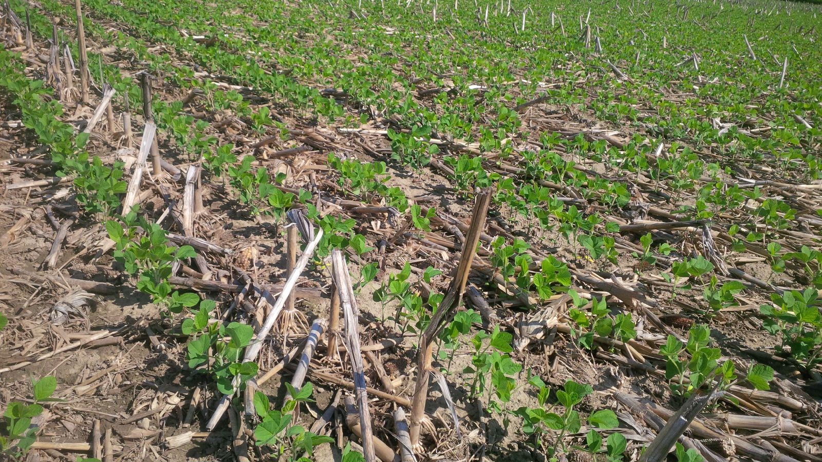

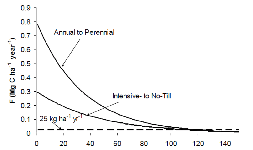


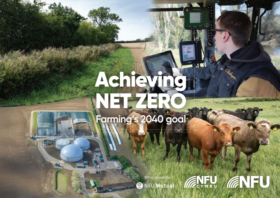


![CFS-banner[1]](https://tdaynard.com/wp-content/uploads/2020/12/cfs-banner1.jpg)


 Without going into details that lie beyond the intended scope of this article, decreases in the energy used to produce electricity in Canada since 2005 have been countered by increases in energy used for road transportation and for oil and gas extraction – with most other GHG-producing sectors showing little change over the 13-year interval.